4 - Evaluating models

Introduction to tidymodels

Looking at predictions

augment(taxi_fit, new_data = taxi_train) %>%
  relocate(tip, .pred_class, .pred_yes, .pred_no)
#> # A tibble: 8,000 × 10
#>    tip   .pred_class .pred_yes .pred_no distance company local dow   month  hour
#>    <fct> <fct>           <dbl>    <dbl>    <dbl> <fct>   <fct> <fct> <fct> <int>
#>  1 yes   yes             0.967   0.0333    17.2  Chicag… no    Thu   Feb      16
#>  2 yes   yes             0.935   0.0646     0.88 City S… yes   Thu   Mar       8
#>  3 yes   yes             0.967   0.0333    18.1  other   no    Mon   Feb      18
#>  4 yes   yes             0.949   0.0507    12.2  Chicag… no    Sun   Mar      21
#>  5 yes   yes             0.821   0.179      0.94 Sun Ta… yes   Sat   Apr      23
#>  6 yes   yes             0.967   0.0333    17.5  Flash … no    Fri   Mar      12
#>  7 yes   yes             0.967   0.0333    17.7  other   no    Sun   Jan       6
#>  8 yes   yes             0.938   0.0616     1.85 Taxica… no    Fri   Apr      12
#>  9 yes   yes             0.938   0.0616     0.53 Sun Ta… no    Tue   Mar      18
#> 10 yes   yes             0.931   0.0694     6.65 Taxica… no    Sun   Apr      11
#> # ℹ 7,990 more rows

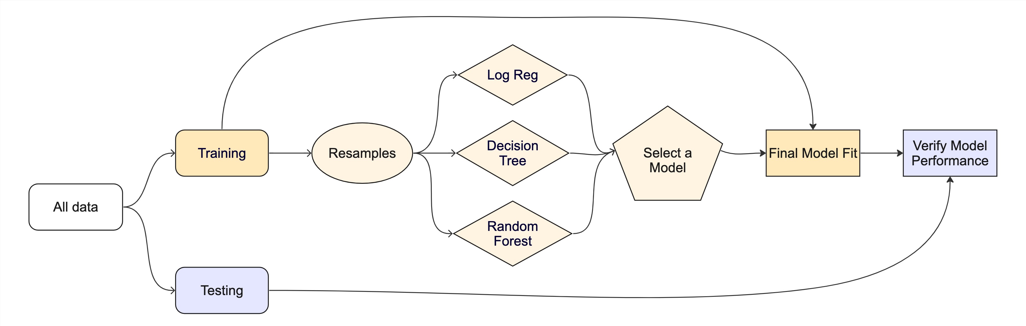
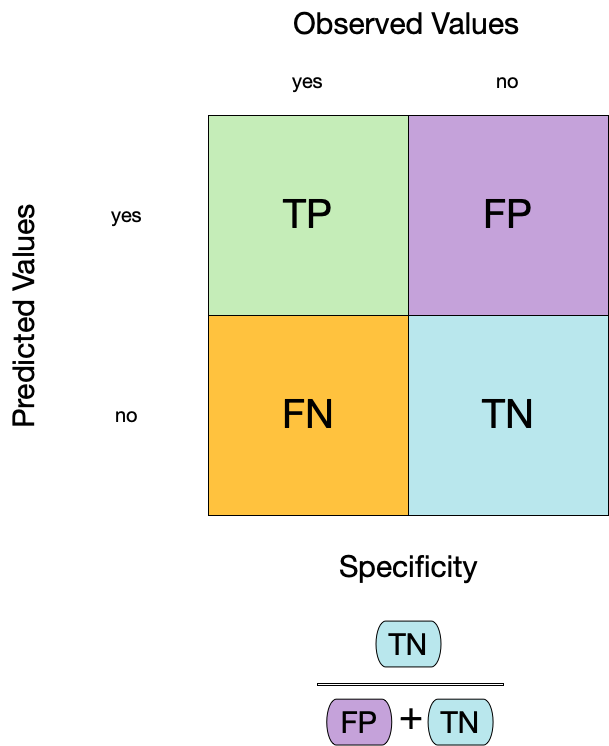
Confusion matrix

augment(taxi_fit, new_data = taxi_train) %>%
  conf_mat(truth = tip, estimate = .pred_class)
#>           Truth
#> Prediction  yes   no
#>        yes 7341  536
#>        no    43   80

Confusion matrix

augment(taxi_fit, new_data = taxi_train) %>%
  conf_mat(truth = tip, estimate = .pred_class) %>%
  autoplot(type = "heatmap")

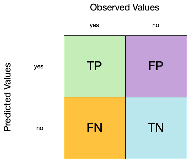
Metrics for model performance

augment(taxi_fit, new_data = taxi_train) %>%
  accuracy(truth = tip, estimate = .pred_class)
#> # A tibble: 1 × 3
#>   .metric  .estimator .estimate
#>   <chr>    <chr>          <dbl>
#> 1 accuracy binary         0.928

Dangers of accuracy

We need to be careful of using accuracy() since it can give “good” performance by only predicting one way with imbalanced data

augment(taxi_fit, new_data = taxi_train) %>%
  mutate(.pred_class = factor("yes", levels = c("yes", "no"))) %>%
  accuracy(truth = tip, estimate = .pred_class)
#> # A tibble: 1 × 3
#>   .metric  .estimator .estimate
#>   <chr>    <chr>          <dbl>
#> 1 accuracy binary         0.923

Metrics for model performance

augment(taxi_fit, new_data = taxi_train) %>%
  sensitivity(truth = tip, estimate = .pred_class)
#> # A tibble: 1 × 3
#>   .metric     .estimator .estimate
#>   <chr>       <chr>          <dbl>
#> 1 sensitivity binary         0.994

Metrics for model performance

augment(taxi_fit, new_data = taxi_train) %>%
  sensitivity(truth = tip, estimate = .pred_class)
#> # A tibble: 1 × 3
#>   .metric     .estimator .estimate
#>   <chr>       <chr>          <dbl>
#> 1 sensitivity binary         0.994

augment(taxi_fit, new_data = taxi_train) %>%
  specificity(truth = tip, estimate = .pred_class)
#> # A tibble: 1 × 3
#>   .metric     .estimator .estimate
#>   <chr>       <chr>          <dbl>
#> 1 specificity binary         0.130

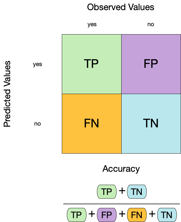
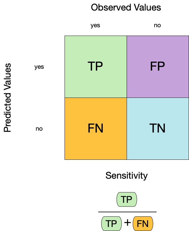
Metrics for model performance

We can use metric_set() to combine multiple calculations into one

taxi_metrics <- metric_set(accuracy, specificity, sensitivity)

augment(taxi_fit, new_data = taxi_train) %>%
  taxi_metrics(truth = tip, estimate = .pred_class)
#> # A tibble: 3 × 3
#>   .metric     .estimator .estimate
#>   <chr>       <chr>          <dbl>
#> 1 accuracy    binary         0.928
#> 2 specificity binary         0.130
#> 3 sensitivity binary         0.994

Metrics for model performance

taxi_metrics <- metric_set(accuracy, specificity, sensitivity)

augment(taxi_fit, new_data = taxi_train) %>%
  group_by(local) %>%
  taxi_metrics(truth = tip, estimate = .pred_class)
#> # A tibble: 6 × 4
#>   local .metric     .estimator .estimate
#>   <fct> <chr>       <chr>          <dbl>
#> 1 yes   accuracy    binary         0.898
#> 2 no    accuracy    binary         0.935
#> 3 yes   specificity binary         0.169
#> 4 no    specificity binary         0.116
#> 5 yes   sensitivity binary         0.987
#> 6 no    sensitivity binary         0.996

Two class data

These metrics assume that we know the threshold for converting “soft” probability predictions into “hard” class predictions.

Is a 50% threshold good?

What happens if we say that we need to be 80% sure to declare an event?

sensitivity ⬇️, specificity ⬆️

What happens for a 20% threshold?

sensitivity ⬆️, specificity ⬇️

Varying the threshold

ROC curves

To make an ROC (receiver operator characteristic) curve, we:

calculate the sensitivity and specificity for all possible thresholds
plot false positive rate (x-axis) versus true positive rate (y-axis)

given that sensitivity is the true positive rate, and specificity is the true negative rate. Hence 1 - specificity is the false positive rate.

We can use the area under the ROC curve as a classification metric:

ROC AUC = 1 💯
ROC AUC = 1/2 😢

ROC curves

# Assumes _first_ factor level is event; there are options to change that
augment(taxi_fit, new_data = taxi_train) %>% 
  roc_curve(truth = tip, .pred_yes) %>%
  slice(1, 20, 50)
#> # A tibble: 3 × 3
#>   .threshold specificity sensitivity
#>        <dbl>       <dbl>       <dbl>
#> 1   -Inf           0         1      
#> 2      0.783       0.209     0.981  
#> 3      1           1         0.00135

augment(taxi_fit, new_data = taxi_train) %>% 
  roc_auc(truth = tip, .pred_yes)
#> # A tibble: 1 × 3
#>   .metric .estimator .estimate
#>   <chr>   <chr>          <dbl>
#> 1 roc_auc binary         0.691

ROC curve plot

augment(taxi_fit, new_data = taxi_train) %>% 
  roc_curve(truth = tip, .pred_yes) %>%
  autoplot()

Your turn

Compute and plot an ROC curve for your current model.

What data are being used for this ROC curve plot?

05:00

⚠️ DANGERS OF OVERFITTING ⚠️

Dangers of overfitting ⚠️

taxi_fit %>%
  augment(taxi_train)
#> # A tibble: 8,000 × 10
#>    .pred_class .pred_yes .pred_no tip   distance company local dow   month  hour
#>    <fct>           <dbl>    <dbl> <fct>    <dbl> <fct>   <fct> <fct> <fct> <int>
#>  1 yes             0.967   0.0333 yes      17.2  Chicag… no    Thu   Feb      16
#>  2 yes             0.935   0.0646 yes       0.88 City S… yes   Thu   Mar       8
#>  3 yes             0.967   0.0333 yes      18.1  other   no    Mon   Feb      18
#>  4 yes             0.949   0.0507 yes      12.2  Chicag… no    Sun   Mar      21
#>  5 yes             0.821   0.179  yes       0.94 Sun Ta… yes   Sat   Apr      23
#>  6 yes             0.967   0.0333 yes      17.5  Flash … no    Fri   Mar      12
#>  7 yes             0.967   0.0333 yes      17.7  other   no    Sun   Jan       6
#>  8 yes             0.938   0.0616 yes       1.85 Taxica… no    Fri   Apr      12
#>  9 yes             0.938   0.0616 yes       0.53 Sun Ta… no    Tue   Mar      18
#> 10 yes             0.931   0.0694 yes       6.65 Taxica… no    Sun   Apr      11
#> # ℹ 7,990 more rows

We call this “resubstitution” or “repredicting the training set”

Dangers of overfitting ⚠️

taxi_fit %>%
  augment(taxi_train) %>%
  accuracy(tip, .pred_class)
#> # A tibble: 1 × 3
#>   .metric  .estimator .estimate
#>   <chr>    <chr>          <dbl>
#> 1 accuracy binary         0.928

We call this a “resubstitution estimate”

Dangers of overfitting ⚠️

taxi_fit %>%
  augment(taxi_train) %>%
  accuracy(tip, .pred_class)
#> # A tibble: 1 × 3
#>   .metric  .estimator .estimate
#>   <chr>    <chr>          <dbl>
#> 1 accuracy binary         0.928

Dangers of overfitting ⚠️

taxi_fit %>%
  augment(taxi_train) %>%
  accuracy(tip, .pred_class)
#> # A tibble: 1 × 3
#>   .metric  .estimator .estimate
#>   <chr>    <chr>          <dbl>
#> 1 accuracy binary         0.928

taxi_fit %>%
  augment(taxi_test) %>%
  accuracy(tip, .pred_class)
#> # A tibble: 1 × 3
#>   .metric  .estimator .estimate
#>   <chr>    <chr>          <dbl>
#> 1 accuracy binary         0.908

⚠️ Remember that we’re demonstrating overfitting

⚠️ Don’t use the test set until the end of your modeling analysis

Your turn

Use augment() and a metric function to compute a classification metric like brier_class().

Compute the metrics for both training and testing data to demonstrate overfitting!

Notice the evidence of overfitting! ⚠️

05:00

Dangers of overfitting ⚠️

taxi_fit %>%
  augment(taxi_train) %>%
  brier_class(tip, .pred_yes)
#> # A tibble: 1 × 3
#>   .metric     .estimator .estimate
#>   <chr>       <chr>          <dbl>
#> 1 brier_class binary        0.0632

taxi_fit %>%
  augment(taxi_test) %>%
  brier_class(tip, .pred_yes)
#> # A tibble: 1 × 3
#>   .metric     .estimator .estimate
#>   <chr>       <chr>          <dbl>
#> 1 brier_class binary        0.0782

What if we want to compare more models?

And/or more model configurations?

And we want to understand if these are important differences?

The testing data are precious 💎

How can we use the training data to compare and evaluate different models? 🤔

Cross-validation

Your turn

If we use 10 folds, what percent of the training data

ends up in analysis
ends up in assessment

for each fold?

03:00

Cross-validation

vfold_cv(taxi_train) # v = 10 is default
#> #  10-fold cross-validation 
#> # A tibble: 10 × 2
#>    splits             id    
#>    <list>             <chr> 
#>  1 <split [7200/800]> Fold01
#>  2 <split [7200/800]> Fold02
#>  3 <split [7200/800]> Fold03
#>  4 <split [7200/800]> Fold04
#>  5 <split [7200/800]> Fold05
#>  6 <split [7200/800]> Fold06
#>  7 <split [7200/800]> Fold07
#>  8 <split [7200/800]> Fold08
#>  9 <split [7200/800]> Fold09
#> 10 <split [7200/800]> Fold10

Cross-validation

What is in this?

taxi_folds <- vfold_cv(taxi_train)
taxi_folds$splits[1:3]
#> [[1]]
#> <Analysis/Assess/Total>
#> <7200/800/8000>
#> 
#> [[2]]
#> <Analysis/Assess/Total>
#> <7200/800/8000>
#> 
#> [[3]]
#> <Analysis/Assess/Total>
#> <7200/800/8000>

Cross-validation

vfold_cv(taxi_train, v = 5)
#> #  5-fold cross-validation 
#> # A tibble: 5 × 2
#>   splits              id   
#>   <list>              <chr>
#> 1 <split [6400/1600]> Fold1
#> 2 <split [6400/1600]> Fold2
#> 3 <split [6400/1600]> Fold3
#> 4 <split [6400/1600]> Fold4
#> 5 <split [6400/1600]> Fold5

Cross-validation

vfold_cv(taxi_train, strata = tip)
#> #  10-fold cross-validation using stratification 
#> # A tibble: 10 × 2
#>    splits             id    
#>    <list>             <chr> 
#>  1 <split [7200/800]> Fold01
#>  2 <split [7200/800]> Fold02
#>  3 <split [7200/800]> Fold03
#>  4 <split [7200/800]> Fold04
#>  5 <split [7200/800]> Fold05
#>  6 <split [7200/800]> Fold06
#>  7 <split [7200/800]> Fold07
#>  8 <split [7200/800]> Fold08
#>  9 <split [7200/800]> Fold09
#> 10 <split [7200/800]> Fold10

Stratification often helps, with very little downside

Cross-validation

We’ll use this setup:

set.seed(123)
taxi_folds <- vfold_cv(taxi_train, v = 10, strata = tip)
taxi_folds
#> #  10-fold cross-validation using stratification 
#> # A tibble: 10 × 2
#>    splits             id    
#>    <list>             <chr> 
#>  1 <split [7200/800]> Fold01
#>  2 <split [7200/800]> Fold02
#>  3 <split [7200/800]> Fold03
#>  4 <split [7200/800]> Fold04
#>  5 <split [7200/800]> Fold05
#>  6 <split [7200/800]> Fold06
#>  7 <split [7200/800]> Fold07
#>  8 <split [7200/800]> Fold08
#>  9 <split [7200/800]> Fold09
#> 10 <split [7200/800]> Fold10

Set the seed when creating resamples

We are equipped with metrics and resamples!

Fit our model to the resamples

taxi_res <- fit_resamples(taxi_wflow, taxi_folds)
taxi_res
#> # Resampling results
#> # 10-fold cross-validation using stratification 
#> # A tibble: 10 × 4
#>    splits             id     .metrics         .notes          
#>    <list>             <chr>  <list>           <list>          
#>  1 <split [7200/800]> Fold01 <tibble [3 × 4]> <tibble [0 × 3]>
#>  2 <split [7200/800]> Fold02 <tibble [3 × 4]> <tibble [0 × 3]>
#>  3 <split [7200/800]> Fold03 <tibble [3 × 4]> <tibble [0 × 3]>
#>  4 <split [7200/800]> Fold04 <tibble [3 × 4]> <tibble [0 × 3]>
#>  5 <split [7200/800]> Fold05 <tibble [3 × 4]> <tibble [0 × 3]>
#>  6 <split [7200/800]> Fold06 <tibble [3 × 4]> <tibble [0 × 3]>
#>  7 <split [7200/800]> Fold07 <tibble [3 × 4]> <tibble [0 × 3]>
#>  8 <split [7200/800]> Fold08 <tibble [3 × 4]> <tibble [0 × 3]>
#>  9 <split [7200/800]> Fold09 <tibble [3 × 4]> <tibble [0 × 3]>
#> 10 <split [7200/800]> Fold10 <tibble [3 × 4]> <tibble [0 × 3]>

Evaluating model performance

taxi_res %>%
  collect_metrics()
#> # A tibble: 3 × 6
#>   .metric     .estimator   mean     n std_err .config             
#>   <chr>       <chr>       <dbl> <int>   <dbl> <chr>               
#> 1 accuracy    binary     0.915     10 0.00309 Preprocessor1_Model1
#> 2 brier_class binary     0.0721    10 0.00245 Preprocessor1_Model1
#> 3 roc_auc     binary     0.624     10 0.0105  Preprocessor1_Model1

We can reliably measure performance using only the training data 🎉

Comparing metrics

How do the metrics from resampling compare to the metrics from training and testing?

taxi_res %>%
  collect_metrics() %>% 
  select(.metric, mean, n)
#> # A tibble: 3 × 3
#>   .metric       mean     n
#>   <chr>        <dbl> <int>
#> 1 accuracy    0.915     10
#> 2 brier_class 0.0721    10
#> 3 roc_auc     0.624     10

The ROC AUC previously was

0.69 for the training set
0.64 for test set

Remember that:

⚠️ the training set gives you overly optimistic metrics

⚠️ the test set is precious

Evaluating model performance

# Save the assessment set results
ctrl_taxi <- control_resamples(save_pred = TRUE)
taxi_res <- fit_resamples(taxi_wflow, taxi_folds, control = ctrl_taxi)

taxi_res
#> # Resampling results
#> # 10-fold cross-validation using stratification 
#> # A tibble: 10 × 5
#>    splits             id     .metrics         .notes           .predictions
#>    <list>             <chr>  <list>           <list>           <list>      
#>  1 <split [7200/800]> Fold01 <tibble [3 × 4]> <tibble [0 × 3]> <tibble>    
#>  2 <split [7200/800]> Fold02 <tibble [3 × 4]> <tibble [0 × 3]> <tibble>    
#>  3 <split [7200/800]> Fold03 <tibble [3 × 4]> <tibble [0 × 3]> <tibble>    
#>  4 <split [7200/800]> Fold04 <tibble [3 × 4]> <tibble [0 × 3]> <tibble>    
#>  5 <split [7200/800]> Fold05 <tibble [3 × 4]> <tibble [0 × 3]> <tibble>    
#>  6 <split [7200/800]> Fold06 <tibble [3 × 4]> <tibble [0 × 3]> <tibble>    
#>  7 <split [7200/800]> Fold07 <tibble [3 × 4]> <tibble [0 × 3]> <tibble>    
#>  8 <split [7200/800]> Fold08 <tibble [3 × 4]> <tibble [0 × 3]> <tibble>    
#>  9 <split [7200/800]> Fold09 <tibble [3 × 4]> <tibble [0 × 3]> <tibble>    
#> 10 <split [7200/800]> Fold10 <tibble [3 × 4]> <tibble [0 × 3]> <tibble>

Evaluating model performance

# Save the assessment set results
taxi_preds <- collect_predictions(taxi_res)
taxi_preds
#> # A tibble: 8,000 × 7
#>    .pred_class .pred_yes .pred_no id      .row tip   .config             
#>    <fct>           <dbl>    <dbl> <chr>  <int> <fct> <chr>               
#>  1 yes             0.938   0.0615 Fold01    14 yes   Preprocessor1_Model1
#>  2 yes             0.946   0.0544 Fold01    19 yes   Preprocessor1_Model1
#>  3 yes             0.973   0.0269 Fold01    33 yes   Preprocessor1_Model1
#>  4 yes             0.903   0.0971 Fold01    43 yes   Preprocessor1_Model1
#>  5 yes             0.973   0.0269 Fold01    74 yes   Preprocessor1_Model1
#>  6 yes             0.903   0.0971 Fold01   103 yes   Preprocessor1_Model1
#>  7 yes             0.915   0.0851 Fold01   104 no    Preprocessor1_Model1
#>  8 yes             0.903   0.0971 Fold01   124 yes   Preprocessor1_Model1
#>  9 yes             0.667   0.333  Fold01   126 yes   Preprocessor1_Model1
#> 10 yes             0.949   0.0510 Fold01   128 yes   Preprocessor1_Model1
#> # ℹ 7,990 more rows

Evaluating model performance

taxi_preds %>% 
  group_by(id) %>%
  taxi_metrics(truth = tip, estimate = .pred_class)
#> # A tibble: 30 × 4
#>    id     .metric  .estimator .estimate
#>    <chr>  <chr>    <chr>          <dbl>
#>  1 Fold01 accuracy binary         0.905
#>  2 Fold02 accuracy binary         0.925
#>  3 Fold03 accuracy binary         0.926
#>  4 Fold04 accuracy binary         0.915
#>  5 Fold05 accuracy binary         0.902
#>  6 Fold06 accuracy binary         0.912
#>  7 Fold07 accuracy binary         0.906
#>  8 Fold08 accuracy binary         0.91 
#>  9 Fold09 accuracy binary         0.918
#> 10 Fold10 accuracy binary         0.931
#> # ℹ 20 more rows

Where are the fitted models?

taxi_res
#> # Resampling results
#> # 10-fold cross-validation using stratification 
#> # A tibble: 10 × 5
#>    splits             id     .metrics         .notes           .predictions
#>    <list>             <chr>  <list>           <list>           <list>      
#>  1 <split [7200/800]> Fold01 <tibble [3 × 4]> <tibble [0 × 3]> <tibble>    
#>  2 <split [7200/800]> Fold02 <tibble [3 × 4]> <tibble [0 × 3]> <tibble>    
#>  3 <split [7200/800]> Fold03 <tibble [3 × 4]> <tibble [0 × 3]> <tibble>    
#>  4 <split [7200/800]> Fold04 <tibble [3 × 4]> <tibble [0 × 3]> <tibble>    
#>  5 <split [7200/800]> Fold05 <tibble [3 × 4]> <tibble [0 × 3]> <tibble>    
#>  6 <split [7200/800]> Fold06 <tibble [3 × 4]> <tibble [0 × 3]> <tibble>    
#>  7 <split [7200/800]> Fold07 <tibble [3 × 4]> <tibble [0 × 3]> <tibble>    
#>  8 <split [7200/800]> Fold08 <tibble [3 × 4]> <tibble [0 × 3]> <tibble>    
#>  9 <split [7200/800]> Fold09 <tibble [3 × 4]> <tibble [0 × 3]> <tibble>    
#> 10 <split [7200/800]> Fold10 <tibble [3 × 4]> <tibble [0 × 3]> <tibble>

🗑️

Alternate resampling schemes

Bootstrapping

set.seed(3214)
bootstraps(taxi_train)
#> # Bootstrap sampling 
#> # A tibble: 25 × 2
#>    splits              id         
#>    <list>              <chr>      
#>  1 <split [8000/2902]> Bootstrap01
#>  2 <split [8000/2916]> Bootstrap02
#>  3 <split [8000/3004]> Bootstrap03
#>  4 <split [8000/2979]> Bootstrap04
#>  5 <split [8000/2961]> Bootstrap05
#>  6 <split [8000/2962]> Bootstrap06
#>  7 <split [8000/3026]> Bootstrap07
#>  8 <split [8000/2926]> Bootstrap08
#>  9 <split [8000/2972]> Bootstrap09
#> 10 <split [8000/2972]> Bootstrap10
#> # ℹ 15 more rows

The whole game - status update

Your turn

Create:

Monte Carlo Cross-Validation sets
validation set

(use the reference guide to find the functions)

Don’t forget to set a seed when you resample!

05:00

Monte Carlo Cross-Validation

set.seed(322)
mc_cv(taxi_train, times = 10)
#> # Monte Carlo cross-validation (0.75/0.25) with 10 resamples  
#> # A tibble: 10 × 2
#>    splits              id        
#>    <list>              <chr>     
#>  1 <split [6000/2000]> Resample01
#>  2 <split [6000/2000]> Resample02
#>  3 <split [6000/2000]> Resample03
#>  4 <split [6000/2000]> Resample04
#>  5 <split [6000/2000]> Resample05
#>  6 <split [6000/2000]> Resample06
#>  7 <split [6000/2000]> Resample07
#>  8 <split [6000/2000]> Resample08
#>  9 <split [6000/2000]> Resample09
#> 10 <split [6000/2000]> Resample10

Validation set

set.seed(853)
taxi_val_split <- initial_validation_split(taxi, strata = tip)
validation_set(taxi_val_split)
#> # A tibble: 1 × 2
#>   splits              id        
#>   <list>              <chr>     
#> 1 <split [6000/2000]> validation

A validation set is just another type of resample

Decision tree 🌳

Random forest 🌳🌲🌴🌵🌴🌳🌳🌴🌲🌵🌴🌲🌳🌴🌳🌵🌵🌴🌲🌲🌳🌴🌳🌴🌲🌴🌵🌴🌲🌴🌵🌲🌵🌴🌲🌳🌴🌵🌳🌴🌳

Random forest 🌳🌲🌴🌵🌳🌳🌴🌲🌵🌴🌳🌵

Ensemble many decision tree models
All the trees vote! 🗳️
Bootstrap aggregating + random predictor sampling

Often works well without tuning hyperparameters (more on this in Advanced tidymodels!), as long as there are enough trees

Create a random forest model

rf_spec <- rand_forest(trees = 1000, mode = "classification")
rf_spec
#> Random Forest Model Specification (classification)
#> 
#> Main Arguments:
#>   trees = 1000
#> 
#> Computational engine: ranger

Create a random forest model

rf_wflow <- workflow(tip ~ ., rf_spec)
rf_wflow
#> ══ Workflow ══════════════════════════════════════════════════════════
#> Preprocessor: Formula
#> Model: rand_forest()
#> 
#> ── Preprocessor ──────────────────────────────────────────────────────
#> tip ~ .
#> 
#> ── Model ─────────────────────────────────────────────────────────────
#> Random Forest Model Specification (classification)
#> 
#> Main Arguments:
#>   trees = 1000
#> 
#> Computational engine: ranger

Your turn

Use fit_resamples() and rf_wflow to:

keep predictions
compute metrics

08:00

Evaluating model performance

ctrl_taxi <- control_resamples(save_pred = TRUE)

# Random forest uses random numbers so set the seed first

set.seed(2)
rf_res <- fit_resamples(rf_wflow, taxi_folds, control = ctrl_taxi)
collect_metrics(rf_res)
#> # A tibble: 3 × 6
#>   .metric     .estimator   mean     n std_err .config             
#>   <chr>       <chr>       <dbl> <int>   <dbl> <chr>               
#> 1 accuracy    binary     0.923     10 0.00317 Preprocessor1_Model1
#> 2 brier_class binary     0.0706    10 0.00243 Preprocessor1_Model1
#> 3 roc_auc     binary     0.616     10 0.0147  Preprocessor1_Model1

The whole game - status update

The final fit

Suppose that we are happy with our random forest model.

Let’s fit the model on the training set and verify our performance using the test set.

We’ve shown you fit() and predict() (+ augment()) but there is a shortcut:

# taxi_split has train + test info
final_fit <- last_fit(rf_wflow, taxi_split) 

final_fit
#> # Resampling results
#> # Manual resampling 
#> # A tibble: 1 × 6
#>   splits              id               .metrics .notes   .predictions .workflow 
#>   <list>              <chr>            <list>   <list>   <list>       <list>    
#> 1 <split [8000/2000]> train/test split <tibble> <tibble> <tibble>     <workflow>

What is in `final_fit`?

collect_metrics(final_fit)
#> # A tibble: 3 × 4
#>   .metric     .estimator .estimate .config             
#>   <chr>       <chr>          <dbl> <chr>               
#> 1 accuracy    binary        0.914  Preprocessor1_Model1
#> 2 roc_auc     binary        0.638  Preprocessor1_Model1
#> 3 brier_class binary        0.0772 Preprocessor1_Model1

These are metrics computed with the test set

What is in `final_fit`?

collect_predictions(final_fit)
#> # A tibble: 2,000 × 7
#>    .pred_class .pred_yes .pred_no id                .row tip   .config          
#>    <fct>           <dbl>    <dbl> <chr>            <int> <fct> <chr>            
#>  1 yes             0.957   0.0426 train/test split     4 yes   Preprocessor1_Mo…
#>  2 yes             0.938   0.0621 train/test split    10 yes   Preprocessor1_Mo…
#>  3 yes             0.958   0.0416 train/test split    19 yes   Preprocessor1_Mo…
#>  4 yes             0.894   0.106  train/test split    23 yes   Preprocessor1_Mo…
#>  5 yes             0.943   0.0573 train/test split    28 yes   Preprocessor1_Mo…
#>  6 yes             0.979   0.0213 train/test split    34 yes   Preprocessor1_Mo…
#>  7 yes             0.954   0.0463 train/test split    35 yes   Preprocessor1_Mo…
#>  8 yes             0.928   0.0722 train/test split    38 yes   Preprocessor1_Mo…
#>  9 yes             0.985   0.0147 train/test split    40 yes   Preprocessor1_Mo…
#> 10 yes             0.948   0.0523 train/test split    42 no    Preprocessor1_Mo…
#> # ℹ 1,990 more rows

What is in `final_fit`?

extract_workflow(final_fit)
#> ══ Workflow [trained] ════════════════════════════════════════════════
#> Preprocessor: Formula
#> Model: rand_forest()
#> 
#> ── Preprocessor ──────────────────────────────────────────────────────
#> tip ~ .
#> 
#> ── Model ─────────────────────────────────────────────────────────────
#> Ranger result
#> 
#> Call:
#>  ranger::ranger(x = maybe_data_frame(x), y = y, num.trees = ~1000,      num.threads = 1, verbose = FALSE, seed = sample.int(10^5,          1), probability = TRUE) 
#> 
#> Type:                             Probability estimation 
#> Number of trees:                  1000 
#> Sample size:                      8000 
#> Number of independent variables:  6 
#> Mtry:                             2 
#> Target node size:                 10 
#> Variable importance mode:         none 
#> Splitrule:                        gini 
#> OOB prediction error (Brier s.):  0.07069778

Use this for prediction on new data, like for deploying

4 - Evaluating models

Looking at predictions

Confusion matrix

Confusion matrix

Confusion matrix

Metrics for model performance

Dangers of accuracy

Metrics for model performance

Metrics for model performance

Metrics for model performance

Metrics for model performance

Two class data

Varying the threshold

ROC curves

ROC curves

ROC curve plot

Your turn

⚠️ DANGERS OF OVERFITTING ⚠️

Dangers of overfitting ⚠️

Dangers of overfitting ⚠️

Dangers of overfitting ⚠️

Dangers of overfitting ⚠️

Dangers of overfitting ⚠️

Dangers of overfitting ⚠️

Your turn

Dangers of overfitting ⚠️

The testing data are precious 💎

How can we use the training data to compare and evaluate different models? 🤔

Cross-validation

Cross-validation

Your turn

Cross-validation

Cross-validation

Cross-validation

Cross-validation

Cross-validation

We are equipped with metrics and resamples!

Fit our model to the resamples

Evaluating model performance

Comparing metrics

Evaluating model performance

Evaluating model performance

Evaluating model performance

Where are the fitted models?

Alternate resampling schemes

Bootstrapping

Bootstrapping

The whole game - status update

Your turn

Monte Carlo Cross-Validation

Validation set

Decision tree 🌳

Random forest 🌳🌲🌴🌵🌴🌳🌳🌴🌲🌵🌴🌲🌳🌴🌳🌵🌵🌴🌲🌲🌳🌴🌳🌴🌲🌴🌵🌴🌲🌴🌵🌲🌵🌴🌲🌳🌴🌵🌳🌴🌳

Random forest 🌳🌲🌴🌵🌳🌳🌴🌲🌵🌴🌳🌵

Create a random forest model

Create a random forest model

Your turn

Evaluating model performance

The whole game - status update

The final fit

What is in final_fit?

What is in final_fit?

What is in final_fit?

The whole game

What is in `final_fit`?

What is in `final_fit`?

What is in `final_fit`?