Extras - Postprocessing
Practical Machine Learning with tidymodels
Startup! ![]()
![]()
![]()



More startup! ![]()

set.seed(429)
class_data <-
  # Nonlinear classification with a low event rate
  sim_classification(5000, intercept = -10) |>
  # Add some noise predictors that are correlated with one another
  bind_cols(sim_noise(5000, num_var = 15, cov_type = "toeplitz", cov_param = 0.5))

sim_split <- initial_split(class_data, prop = 0.75, strata = class)
sim_train <- training(sim_split)
sim_test  <- testing(sim_split)

set.seed(523)
sim_rs <- vfold_cv(sim_train, v = 10, strata = class)
Our neural network model ![]()
![]()
![]()
![]()




rec <-
  recipe(class ~ ., data = sim_train) |>
  step_normalize(all_numeric_predictors())

nnet_spec <-
  mlp(hidden_units = tune(), penalty = tune(), learn_rate = tune(),
      epochs = 100, activation = tune()) |>
  # Remove the class_weights argument
  set_engine("brulee", stop_iter = 10) |>
  set_mode("classification")

nnet_wflow <- workflow(rec, nnet_spec)

nnet_param <-
  nnet_wflow |>
extract_parameter_set_dials() Tailors ![]()
The tailor package is similar to recipes but specifies how to adjust predictions.
A simple example:
Like a recipe, this initial call doesn’t do anything but declare intent.
Unlike a recipe, it does not need the data (i.e., predictions) at this point.
- Relevant prediction columns are selected when
fit()is used (next slide).
- Relevant prediction columns are selected when
Manual use of a tailor ![]()
There is a fit() method that requires data and the names of the prediction columns:
three_rows <-
  tribble(
     ~ class, ~ .pred_class, ~.pred_class_1, ~.pred_class_2,
   "class_1",     "class_1",            0.6,            0.4,
   "class_1",     "class_2",            0.4,            0.6,
   "class_2",     "class_2",            0.1,            0.9
  ) |>
  mutate(across(where(is.character), factor))

thrsh_fit <-
  thrsh_tlr |>
  fit(
    three_rows,
    outcome = class,
    estimate = .pred_class,
    .pred_class_1:.pred_class_2  # No argument name and order matches factor levels
  )
Manual use of a tailor ![]()
predict() applies the adjustments:
tailors within workflows ![]()
![]()

In practice, we would add the tailor to a workflow to make it easier to use:
- We don’t have to set the names of the outcome or prediction columns (yet).
fit()andpredict()happen automatically.
Tuning the probability threshold ![]()
![]()
![]()
![]()

Tuning the probability threshold ![]()
![]()

Nearly the same code as before:
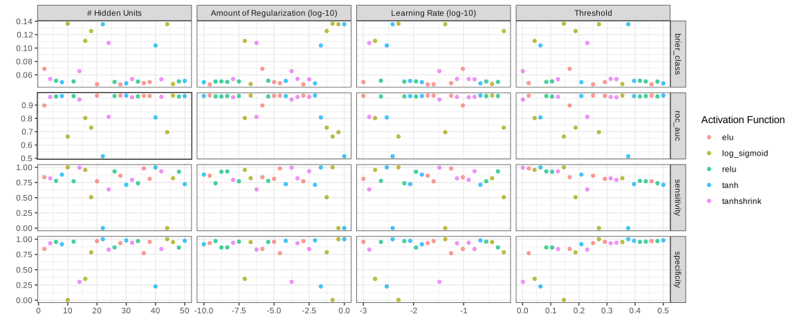
Grid results ![]()
Multimetric optimization ![]()
nnet_thrsh_res |>
  show_best_desirability(
    maximize(sensitivity),
    minimize(brier_class),
    constrain(specificity, low = 0.8, high = 1.0)
  ) |>
  relocate(threshold, sensitivity, specificity, brier_class, .d_overall)
#> # A tibble: 5 × 14
#>   threshold sensitivity specificity brier_class .d_overall hidden_units  penalty
#>       <dbl>       <dbl>       <dbl>       <dbl>      <dbl>        <int>    <dbl>
#> 1    0.0842       0.932       0.866      0.0495      0.964           26 4.64e- 9
#> 2    0.105        0.926       0.864      0.0503      0.959           48 1.78e- 9
#> 3    0.250        0.861       0.936      0.0458      0.952           28 2.61e-10
#> 4    0.126        0.934       0.838      0.0535      0.949           42 3.16e- 3
#> 5    0.209        0.879       0.918      0.0491      0.947            8 1   e-10
#> # ℹ 7 more variables: activation <chr>, learn_rate <dbl>, .config <chr>,
#> #   roc_auc <dbl>, .d_max_sensitivity <dbl>, .d_min_brier_class <dbl>,
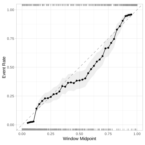
#> # .d_box_specificity <dbl>Calibration![]()
![]()
more_sens <-
  nnet_thrsh_res |>
  select_best_desirability(
    maximize(sensitivity),
    minimize(brier_class),
    constrain(specificity, low = 0.8, high = 1.0)
  )

nnet_thrsh_res |>
  collect_predictions(
    parameters = more_sens
  ) |>
  cal_plot_windowed(
    truth = class,
    estimate = .pred_class_1,
    window_size = 0.2,
    step_size = 0.025,
  )
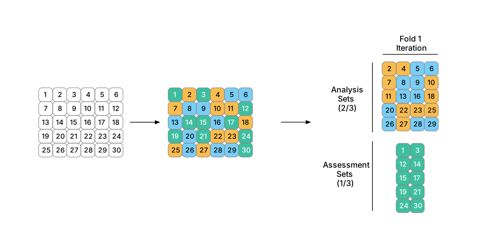
Example: 3-fold CV
Example: 3-fold CV internal split