7 - Feature selection

Practical Machine Learning with tidymodels

Startup!

library(tidymodels)
library(important)
library(probably)
library(mirai)

tidymodels_prefer()
theme_set(theme_bw())
options(pillar.advice = FALSE, pillar.min_title_chars = Inf)
daemons(parallel::detectCores())

More startup!

set.seed(429)
class_data <- 
  # Nonlinear classification with a low event rate
  sim_classification(5000, intercept = -10) |> 
  # Add some noise predictors that are correlated with one another
  bind_cols(sim_noise(5000, num_var = 15, cov_type = "toeplitz", cov_param = 0.5))

sim_split <- initial_split(class_data, prop = 0.75, strata = class)
sim_train <- training(sim_split)
sim_test  <- testing(sim_split)

set.seed(523)
sim_rs <- vfold_cv(sim_train, v = 10, strata = class)

Why remove features/predictors?

Models and feature selection

Some models automatically remove predictors by never using them in the model:

tree- and rule-based models
some regularized models (e.g., glmnet)
multivariate adaptive regression splines (MARS)
RuleFit
not really ensembles though

Sometimes using irrelevant predictors hurts model performance.

Effects of extra predictors

AML4TD

General selection methods

wrappers: a sequential algorithm proposes feature subsets, fits the model with these subsets, and then determines a better subset from the results.
filters: screen predictors before adding them to the model.

tidymodels doesn’t have any wrappers (but see the caret documentation for them)

The new important package does have filters via recipes.

Be careful!!!

tidymodels has always contained some “hidden guardrails” that should prevent practitioners from making subtle (but consequential) methodological mistakes.

Feature selection is a good example. Based on the literature, it is easily done wrong.

The selection process should take place inside a resampling loop so that the workflow does not overfit the predictors.

A&M (2002), AML4TD, FES

Imbalanced example

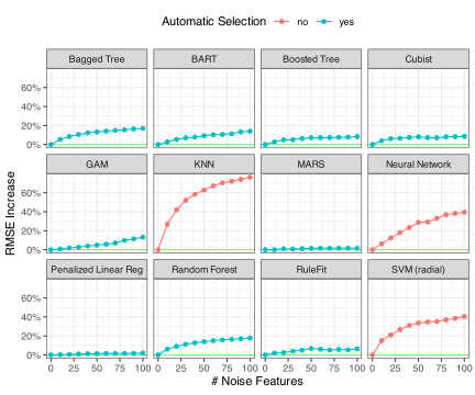
IMPORTANT

We released two packages this year that enable supervised feature selection:

filtro: low-level scoring methods for predictors (e.g., importance).
important: tools for permutation importance and recipes steps for supervised feature selection.

Let’s look at the help page for important::step_predictor_best().

K-nearest neighbors

rec <-
  recipe(class ~ ., data = sim_train) |>
  step_predictor_best(
    all_predictors(),
    score = "imp_rf",
    prop_terms = tune(),
    id = "filter"
  ) |>
  step_normalize(all_numeric_predictors())
  
knn_spec <- 
  nearest_neighbor(neighbors = tune(), weight_func = tune()) |> 
  set_mode("classification")
  
thrsh_tlr <-
  tailor() |>
  adjust_probability_threshold(threshold = tune())

Setup the workflow

knn_wflow <- workflow(rec, knn_spec, thrsh_tlr)

knn_param <-
  knn_wflow |>
  extract_parameter_set_dials() |>
  update(
    threshold = threshold(c(0.001, 0.1)),
    neighbors = neighbors(c(1, 50)),
    prop_terms = prop_terms(c(0.1, 1))
  )

Tuning results

cls_mtr <- metric_set(brier_class, roc_auc, sensitivity, specificity)
ctrl <- control_grid(save_pred = TRUE, save_workflow = TRUE)

set.seed(12)
knn_res <-
  knn_wflow |>
  tune_grid(
    resamples = sim_rs,
    grid = 20,
    control = ctrl,
    metrics = cls_mtr,
    param_info = knn_param
  )

Grid results

autoplot(knn_res)

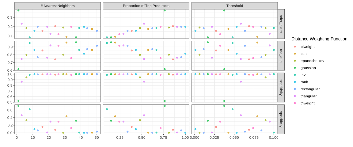
Brier results

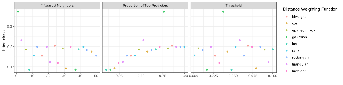
autoplot(knn_res, metric = "brier_class") + 
  facet_grid(. ~ name, scale = "free_x")

ROC curve results

autoplot(knn_res, metric = "roc_auc") + 
  facet_grid(. ~ name, scale = "free_x")

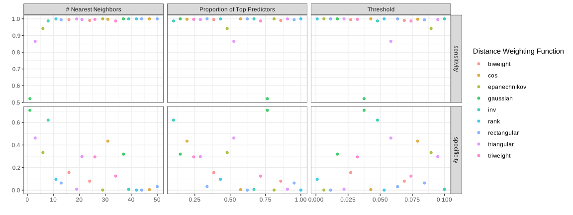
Sensitivity/Specificity results

autoplot(knn_res, metric = c("sensitivity", "specificity"))

Fit the model and get filter information

knn_fit <- fit_best(knn_res, metric = "brier_class")
filter_info <-
    knn_fit |>
    extract_recipe() |>
    tidy(id = "filter")

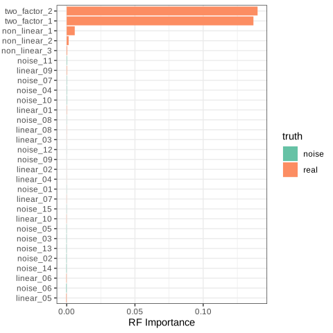
filter_info
#> # A tibble: 30 × 4
#>    terms        removed      score id    
#>    <chr>        <lgl>        <dbl> <chr> 
#>  1 two_factor_1 FALSE    0.137     filter
#>  2 two_factor_2 FALSE    0.140     filter
#>  3 non_linear_1 FALSE    0.00591   filter
#>  4 non_linear_2 TRUE     0.00144   filter
#>  5 non_linear_3 TRUE     0.000402  filter
#>  6 linear_01    TRUE     0.000163  filter
#>  7 linear_02    TRUE    -0.0000237 filter
#>  8 linear_03    TRUE     0.0000385 filter
#>  9 linear_04    TRUE    -0.0000384 filter
#> 10 linear_05    TRUE    -0.000333  filter
#> # ℹ 20 more rows

The truth about our data

The data were simulated and 15 out of 30 predictors were uninformative (and highly correlated). How did we do?

	noise	real
kept	0	3
removed	15	12

selection sensitivity: 20%
selection specificity: 100%

It was good at removing noise but not keeping the real predictors.

Random forest importance scores

# A "truth" column was added
filter_info |>
  mutate(
    terms = factor(terms),
    terms = reorder(terms, score)
  ) |>
  ggplot(
    aes(x = score, 
        y = terms, 
        fill = truth)
  ) +
  geom_bar(stat = "identity") + 
  labs(x = "RF Importance", y = NULL) + 
  scale_fill_brewer(palette = "Set2")

The simulation

The simulation system is documented here with method = "caret". The two most important predictors being retained correspond to:

# In logit units: 
- 4 * two_factor_1 + 4 * two_factor_2 + 2 * two_factor_1 * two_factor_2

Most of the others are small linear effects and tree-based models are not great at modeling those.

Also, the noise predictors were simulated to have fairly high correlations with one another. That can often compromise random forest importance scores.

Other steps

The important package has two other feature selection steps that can be used with multiple scores:

step_predictor_retain(): choose predictors based on a logical statement. Example:

imp_rf > 2 & cor_pearson >= 0.75

step_predictor_desirability(): choose multiple scores to compute then use desirability functions to rank them:

desirability(
  maximize(correlation),
  maximize(imp_rf)
)

Proceed to the test set

Manual approach

We already have our fitted model and, if we are happy with it:

test_pred <- augment(knn_fit, sim_test)
test_pred |> cls_mtr(class, estimate = .pred_class, .pred_class_1)
#> # A tibble: 4 × 3
#>   .metric     .estimator .estimate
#>   <chr>       <chr>          <dbl>
#> 1 sensitivity binary         1    
#> 2 specificity binary         0.613
#> 3 brier_class binary         0.262
#> 4 roc_auc     binary         0.937

Resampling estimates:

#> # A tibble: 4 × 4
#>   .metric       mean     n std_err
#>   <chr>        <dbl> <int>   <dbl>
#> 1 sensitivity 0.987     10 0.00319
#> 2 specificity 0.620     10 0.0169 
#> 3 brier_class 0.0854    10 0.00220
#> 4 roc_auc     0.951     10 0.00212

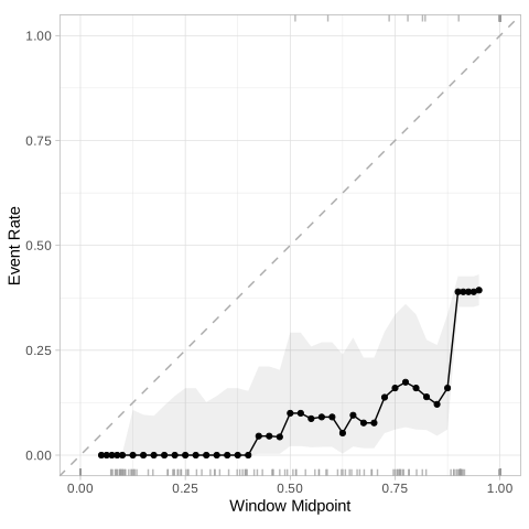
Checking (Approximate) Calibration

test_pred|>
  cal_plot_windowed(
    truth = class,
    estimate = .pred_class_1,
    window_size = 0.2,
    step_size = 0.025,
  )

Looks alright. The small effective sample size (0 events) makes it pretty noisy.

Automated approach

Similar to fit_best(), there is a convenience function that can be used to get the final model and the test set results.

We have to start with a finalized workflow (i.e., no tune() values):

knn_best <- select_best(knn_res, metric = "brier_class")
knn_last_wflow <- finalize_workflow(knn_wflow, knn_best)

Automated approach

last_fit() uses the original split object to fit, predict, and measure the model using the test set:

knn_test_res <- 
  knn_last_wflow |> 
  last_fit(sim_split, metrics = cls_mtr)
  
knn_test_res
#> # Resampling results
#> # Manual resampling 
#> # A tibble: 1 × 6
#>   splits              id               .metrics .notes   .predictions .workflow 
#>   <list>              <chr>            <list>   <list>   <list>       <list>    
#> 1 <split [3749/1251]> train/test split <tibble> <tibble> <tibble>     <workflow>

Automated approach

We can pick out the parts that we want:

knn_final_fit <- knn_test_res |> extract_workflow()
knn_test_pred <- knn_test_res |> collect_predictions()
knn_test_mtr  <- knn_test_res |> collect_metrics()

knn_test_mtr
#> # A tibble: 4 × 4
#>   .metric     .estimator .estimate .config        
#>   <chr>       <chr>          <dbl> <chr>          
#> 1 sensitivity binary        0.936  pre0_mod0_post0
#> 2 specificity binary        0.825  pre0_mod0_post0
#> 3 brier_class binary        0.0485 pre0_mod0_post0
#> 4 roc_auc     binary        0.946  pre0_mod0_post0

Easy peasy!