4 - Feature engineering: dummies and embeddings

Getting More Out of Feature Engineering and Tuning for Machine Learning

Getting set up

library(tidymodels)
library(embed)
library(extrasteps)

tidymodels_prefer()
theme_set(theme_bw())
options(pillar.advice = FALSE, pillar.min_title_chars = Inf)

# Load our example data for this section
"https://github.com/tidymodels/workshops/raw/refs/heads/2025-GMOFETML/slides/leaf_data.RData" |> 
  url() |> 
  load()

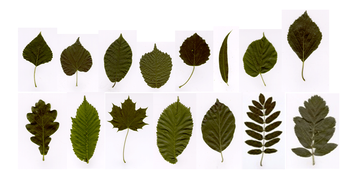
Leaf data

Leaf data set

Slightly modified version of modeldata::leaf_id_flavia.

glimpse(leaf_data)
#> Rows: 1,907
#> Columns: 55
#> $ species                    <fct> chinese_redbud, chinese_redbud, chinese_red…
#> $ apex                       <fct> none, none, none, none, none, none, none, n…
#> $ base                       <fct> none, none, none, none, none, none, none, n…
#> $ shape                      <fct> heart_shape, heart_shape, heart_shape, hear…
#> $ edge                       <chr> "smooth", "smooth", "smooth", "smooth", "sm…
#> $ outlying_polar             <dbl> 0, 0, 0, 0, 0, 0, 0, 0, 0, 0, 0, 0, 0, 0, 0…
#> $ skewed_polar               <dbl> 0.4610066, 0.4747877, 0.5356883, 0.4771338,…
#> $ clumpy_polar               <dbl> 0.006479784, 0.011100482, 0.017317486, 0.01…
#> $ sparse_polar               <dbl> 0.01449941, 0.01451566, 0.02953578, 0.01425…
#> $ striated_polar             <dbl> 0.9788360, 0.9797980, 0.6758621, 0.9896373,…
#> $ convex_polar               <dbl> 0.000899987, 0.000152532, 0.035230741, 0.00…
#> $ skinny_polar               <dbl> 0.1177954, 0.5440493, 0.7764908, 0.7067394,…
#> $ stringy_polar              <dbl> 1.0000000, 1.0000000, 0.8544140, 1.0000000,…
#> $ monotonic_polar            <dbl> 0.026807610, 0.005554220, 0.068481538, 0.09…
#> $ outlying_contour           <dbl> 0, 0, 0, 0, 0, 0, 0, 0, 0, 0, 0, 0, 0, 0, 0…
#> $ skewed_contour             <dbl> 0.4954035, 0.5321818, 0.5451171, 0.4675013,…
#> $ clumpy_contour             <dbl> 0.007898114, 0.010846498, 0.020271493, 0.01…
#> $ sparse_contour             <dbl> 0.01449941, 0.01436114, 0.02903878, 0.01451…
#> $ striated_contour           <dbl> 0.9744898, 0.9811321, 0.6766917, 0.9784946,…
#> $ convex_contour             <dbl> 0.000479470, 0.000000000, 0.035908221, 0.00…
#> $ skinny_contour             <dbl> 0.1810093, 1.0000000, 0.7806988, 0.1348225,…
#> $ stringy_contour            <dbl> 1.0000000, 1.0000000, 0.8864787, 1.0000000,…
#> $ monotonic_contour          <dbl> 0.000816260, 0.000008740, 0.001253195, 0.32…
#> $ num_max_points             <dbl> 1, 3, 4, 1, 1, 1, 1, 1, 1, 1, 1, 1, 1, 6, 1…
#> $ num_min_points             <dbl> 2, 4, 7, 1, 1, 1, 1, 1, 1, 1, 1, 2, 2, 8, 2…
#> $ diameter                   <dbl> 1255.830, 1227.826, 1113.228, 1219.185, 118…
#> $ area                       <dbl> 936626.5, 917300.5, 855376.5, 901303.0, 885…
#> $ perimeter                  <dbl> 3830.534, 3781.445, 3695.646, 3678.409, 383…
#> $ physiological_length       <dbl> 1253, 1218, 1098, 1205, 1153, 1179, 1188, 1…
#> $ physiological_width        <dbl> 1088, 1091, 1083, 1053, 1078, 1073, 1054, 1…
#> $ aspect_ratio               <dbl> 0.8683160, 0.8957307, 0.9863388, 0.8738589,…
#> $ rectangularity             <dbl> 0.6870470, 0.6903027, 0.7193273, 0.7103222,…
#> $ circularity                <dbl> 0.8021540, 0.8061315, 0.7870211, 0.8370680,…
#> $ compactness                <dbl> 15.66578, 15.58849, 15.96701, 15.01237, 16.…
#> $ narrow_factor              <dbl> 1.154255, 1.125413, 1.027912, 1.157821, 1.1…
#> $ perimeter_ratio_diameter   <dbl> 3.050202, 3.079790, 3.319756, 3.017104, 3.2…
#> $ perimeter_ratio_length     <dbl> 3.520711, 3.466036, 3.412416, 3.493266, 3.5…
#> $ perimeter_ratio_lw         <dbl> 1.636281, 1.637698, 1.694473, 1.629056, 1.7…
#> $ num_convex_points          <dbl> 125, 128, 114, 138, 125, 125, 121, 112, 115…
#> $ perimeter_convexity        <dbl> 0.9404967, 0.9393550, 0.9232549, 0.9502414,…
#> $ area_convexity             <dbl> 0.02359372, 0.03175513, 0.03932713, 0.01740…
#> $ area_ratio_convexity       <dbl> 0.9769501, 0.9692222, 0.9621610, 0.9828892,…
#> $ equivalent_diameter        <dbl> 1092.0393, 1080.7142, 1043.5992, 1071.2491,…
#> $ eccentricity               <dbl> 0.44400376, 0.26866788, 0.31952502, 0.44811…
#> $ contrast                   <dbl> 38.69163, 32.73154, 23.20849, 30.14546, 23.…
#> $ correlation_texture        <dbl> 0.9959609, 0.9967740, 0.9975354, 0.9968981,…
#> $ inverse_difference_moments <dbl> 0.5951133, 0.6022763, 0.6363508, 0.6135506,…
#> $ entropy                    <dbl> 6.291552, 6.273267, 5.764995, 6.203471, 5.9…
#> $ mean_red_val               <dbl> 38.02429, 34.55425, 30.92509, 33.44151, 33.…
#> $ mean_green_val             <dbl> 72.38449, 69.89448, 69.22250, 71.32743, 70.…
#> $ mean_blue_val              <dbl> 42.78902, 42.93044, 40.80089, 40.73282, 42.…
#> $ std_red_val                <dbl> 41.66486, 40.48649, 38.55110, 39.09408, 40.…
#> $ std_green_val              <dbl> 74.26665, 73.05275, 76.77596, 75.85529, 75.…
#> $ std_blue_val               <dbl> 46.36232, 48.04195, 48.09177, 46.57170, 48.…
#> $ correlation                <dbl> -0.027629688, -0.003103965, -0.036341630, 0…

Leaf data set

Your turn

Load and explore the leaf data

Make time to look at the edge column and think about how one would encode it into numerics

05:00

Leaf edges

Low number of unique levels
Some overlap

leaf_data |>
  count(edge)
#> # A tibble: 7 × 2
#>   edge                 n
#>   <chr>            <int>
#> 1 ""                  62
#> 2 "denate"            65
#> 3 "lobed"            109
#> 4 "lobed, smooth"     52
#> 5 "lobed, toothed"   109
#> 6 "smooth"          1204
#> 7 "toothed"          306

Advanced Dummies

Leaf edges dummies

(technically one-hot encoding)

lobed	lobed..toothed	smooth	toothed
0	1	0	0
0	0	0	1
0	0	1	0
0	0	1	0
0	0	0	1
1	0	0	0

Dummy variables

Pros

Commonly used
Easy interpretation
Will rarely lead to a decrease in performance

Cons

Can create many columns
Needs clean levels
Not likely the most efficient representation

Overlapping

Some of the labels

lobed
smooth
toothed
lobed, smooth
lobed, toothed

If you want to find a “toothed” leaf, which level do you pick?

toothed
lobed, toothed
toothed and lobed, toothed

We can let lobed, toothed be counted for lobed and toothed

Advanced Dummies

This is basically a poor man’s Natural Language Processing.

tokenization -> counting

We think it is a frequent enough case that it is considered its own method.

We have 2 variants: “extraction” and “multi choice”

Advanced Dummies - Extraction

Works on a singular column, using a regular expression to extract the items we want to count.

Done using regular expressions, either by specifying sep to split the string by, or by using pattern to extract the items.

Allows for 0 to many items in each string.

Implemented as step_dummy_extract().

FEAZ

Advanced Dummies - Extraction

Input

""
"denate"
"lobed"
"lobed, smooth"
"lobed, toothed"
"smooth"
"toothed"

Using

sep = ", "

Result

denate	lobed	smooth	toothed
0	0	0	0
1	0	0	0
0	1	0	0
0	1	1	0
0	1	0	1
0	0	1	0
0	0	0	1

Advanced Dummies - Extraction

Input

"Etching on paper"
"Oil paint on canvas"
"Acrylic paint on paper"
"Oil paint and wax on canvas"
"Oil paint, ink on canvas"

Using

sep = ", "

Result

Acrylic.paint.on.paper	Etching.on.paper	ink.on.canvas	Oil.paint	Oil.paint.and.wax.on.canvas	Oil.paint.on.canvas
0	1	0	0	0	0
0	0	0	0	0	1
1	0	0	0	0	0
0	0	0	0	1	0
0	0	1	1	0	0

Advanced Dummies - Extraction

Input

"Etching on paper"
"Oil paint on canvas"
"Acrylic paint on paper"
"Oil paint and wax on canvas"
"Oil paint, ink on canvas"

Using

sep = "(, )|( and )|( on )"

Result

Acrylic.paint	canvas	Etching	ink	Oil.paint	paper	wax
0	0	1	0	0	1	0
0	1	0	0	1	0	0
1	0	0	0	0	1	0
0	1	0	0	1	0	1
0	1	0	1	1	0	0

Advanced Dummies - Extraction

Input

"['red', 'blue']"
"['red', 'blue', 'white']"
"['blue', 'blue', 'blue']"

Using

pattern = "(?<=')[^',]+(?=')"

Result

blue	red	white
1	1	0
1	1	1
3	0	0

Advanced Dummies - Multi Choice

Works on multiple columns, counting items across columns.

It can be seen as joining multiple applications of dummy variables together.

Allows for 0 to many items.

Implemented as step_dummy_multi_choice().

FEAZ

Advanced Dummies - Multi Choice

Input

lang_1	lang_2	lang_3
English	NA	Italian
Spanish	French	French
NA	NA	NA
English	NA	NA

Result

English	French	Italian	Spanish
1	0	1	0
0	1	0	1
0	0	0	0
1	0	0	0

Othering

Both step_dummy_extract() and step_dummy_multi_choice() contain a threshold argument.

This is used to combine infrequent levels together.

We have a step step_other() that does this for nominal variables, but it doesn’t work in these cases, as it has to happen after the extraction/combination.

Othering

threshold = 0 produces 1217 columns.

canvas	colour	Etching	monitor.or.projection	Oil.paint	paper	sound..stereo.	Video
0	1	0	1	0	0	1	1
0	0	1	0	0	1	0	0
0	0	1	0	0	1	0	0
0	0	1	0	0	1	0	0
1	0	0	0	1	0	0	0
1	0	0	0	1	0	0	0

Othering

threshold = 0.05 produces 11 columns.

canvas	colour	Etching	paper	other
0	1	0	0	3
0	0	1	1	0
0	0	1	1	0
0	0	1	1	0
1	0	0	0	1
1	0	0	0	1

Your turn

Figure out whether step_dummy_extract() or step_dummy_multi_choice() is most appropriate on the edge variable in leaf_data and apply it

03:00

Dimensionality Reduction

What is it?

Techniques that remove or alter features in order to have fewer but more informative features.

Why do we do it?

redundant information
ineffective representation
computational speed

Redundant Information

A feature with no information could be included.

leaf_data |>
  count(outlying_contour)
#> # A tibble: 1 × 2
#>   outlying_contour     n
#>              <dbl> <int>
#> 1                0  1907

Redundant Information

Ineffective Representation

While keeping our models in mind, we want to make sure the data is well-suited

Correlated data
- hard for some models
lat/lon compared to distance/angle
- hard for most models

Ineffective Representation

Computational Speed

Depending on what method we are using and how the data is affected by it, we could see a large reduction in features. This, in turn, leads to a smaller model that is faster to train on.

Only exploration and trial and error can determine whether you should use dimensionality reduction techniques. Knowing which methods do what helps you determine what to try.

Dimensionality Reduction Method

Zero Variance removal
PCA
- Truncated PCA
- Sparse PCA
NNMF
UMAP
Isomap

Restrictions

All the methods shown today will not be able to handle

missing data
Non-numeric data

Why not t-SNE?

One of the main requirements for a feature engineering method is that you can reapply the trained transformation done on the training data set to the testing data set.

This is not possible with t-SNE as it is an iterative method that shifts observations in the lower-dimensional space based on their distances to points in the higher-dimensional space.

It doesn’t create a mapping that can be reused.

PCA

Principal Compoment Analysis is a linear combination of the original data such that most of the variation is captured in the first variable, then the second, then the third, and so on.

FEAZ, FES

PCA Algorithm

The first principal component of a set of features \(X_1, X_2, ..., X_p\) is the normalized linear combination of the features.

\[ Z_1 = \phi_{11} X_1 + \phi_{21} X_2 + ... + \phi_{p1}X_p \]

that has the largest variance under the constraint that \(\sum_{j=1}^p \phi_{j1}^2 = 1\).

we refer to \(\phi_{11}, ..., \phi_{p1}\) as the loadings of the first principal component.

And think of them as the loading vector \(\phi_1\).

PCA Algorithm

since we have \(z_{i1} = \phi_{11} x_{i1} + \phi_{21} x_{i2} + ... + \phi_{p1}x_{ip}\), then we can write

\[ \underset{\phi_{11}, ..., \phi_{p1}}{\text{maximize}} \left\{ \dfrac{1}{n} \sum^n_{i=j} z_{i1} ^2 \right\} \quad \text{subject to} \quad \sum_{j=1}^p \phi_{j1}^2 = 1 \]

We are, in essence, maximizing the sample variance of the \(n\) values of \(z_{i1}\).

We refer to \(z_{11}, ..., z_{n1}\) as the scores of the first principal component.

PCA Algorithm

Luckily, this can be solved using techniques from Linear Algebra, more specifically, it can be solved using an eigen decomposition.

One of the main strengths of PCA is that you don’t need to use optimization to get the results without approximations.

PCA Algorithm

Once the first principal component is calculated, we can calculate the second principal component.

We find the second principal component \(Z_2\) as a linear combination of \(X_1, ..., X_p\) that has the maximal variance out of the linear combinations that are uncorrelated with \(Z_1\)

this is the same as saying that \(\phi_2\) should be orthogonal to the direction \(\phi_1\)

How is that a dimensionality reduction method?

By itself, it isn’t, as it rotates all the features in the feature space.

It becomes a dimensionality reduction method if we only calculate some of the principal components.

This is typically done by retaining a specific number of components or as a threshold on the variance explained.

4 different percent variance plots

Faceted bar chart. 4 bar charts in a 2 by 2 grid. Each one represents a different data set which has had PCA applied to it.

Applying PCA with recipes

Either use the num_comp argument.

rec <- recipe(mpg ~ ., data = mtcars) |>
  step_normalize(all_predictors()) |>
  step_pca(all_numeric_predictors(), num_comp = 5)

or using the threshold argument

rec <- recipe(mpg ~ ., data = mtcars) |>
  step_normalize(all_predictors()) |>
  step_pca(all_numeric_predictors(), threshold = 0.8)

Your turn

Apply PCA using step_pca() to leaf_data data set.

Experiment with different values of num_comp and or threshold.

05:00

PCA Pros and Cons

Pros

Fast
Reliable
Exact results (up to sign changes)

Cons

Computational time is linear in the number of columns
Can be quite hard to interpret

Truncated PCA

Computational time is linear in the number of columns

By default, step_pca() calculates all the loading vectors. And then subset them down to what you need.

Instead, we can use a different implementation that only calculates what you need. This is what we call truncated PCA.

FEAZ

Truncated PCA with recipes

Can only be done using num_comp

library(embed)

rec <- recipe(mpg ~ ., data = mtcars) |>
  step_normalize(all_predictors()) |>
  step_pca_truncated(all_numeric_predictors(), num_comp = 5)

Sparse PCA

Can be quite hard to interpret

Every component is a linear combination of all predictors.

\[ \begin{alignat}{4} PC1 &= cyl \cdot -0.021 &&+ disp \cdot -0.85 &&+ hp \cdot -0.52\\ PC2 &= cyl \cdot 0.013 &&+ disp \cdot -0.52 &&+ hp \cdot 0.85\\ PC3 &= cyl \cdot -0.12 &&+ disp \cdot 0.016 &&+ hp \cdot 0.081\\ PC4 &= cyl \cdot -0.22 &&+ disp \cdot -0.0061 &&+ hp \cdot 0.033\\ PC5 &= cyl \cdot 0.73 &&+ disp \cdot -0.014 &&+ hp \cdot 0.0016 \end{alignat} \]

If we could force some of the loadings to be 0, it would reduce things a lot.

FEAZ

Sparse PCA with recipes

Can only be done using num_comp.

The predictor_prop argument is used to determine how many zeroes in the loadings.

library(embed)

rec <- recipe(mpg ~ ., data = mtcars) |>
  step_normalize(all_predictors()) |>
  step_pca_sparse(all_numeric_predictors(), num_comp = 5, predictor_prop = 0.8)

Sparse PCA with recipes

predictor_prop = 0.8

recipe(mpg ~ ., data = mtcars) |>
  step_normalize(all_predictors()) |>
  step_pca_sparse(all_numeric_predictors(), num_comp = 4, predictor_prop = 0.8) |>
  prep() |>
  tidy(number = 2) |>
  pivot_wider(names_from = component, values_from = value) |>
  select(-id)
#> # A tibble: 10 × 5
#>    terms      PC1    PC2     PC3      PC4
#>    <chr>    <dbl>  <dbl>   <dbl>    <dbl>
#>  1 cyl   -0.503    0      0.0755  0      
#>  2 disp  -0.504    0      0       0.227  
#>  3 hp    -0.377   -0.228 -0.0985  0      
#>  4 drat   0.267   -0.262  0       0.911  
#>  5 wt    -0.420    0.105 -0.383   0.236  
#>  6 qsec   0        0.473 -0.425   0.0966 
#>  7 vs     0.313    0.203 -0.429  -0.0774 
#>  8 am     0.0687  -0.440  0.191  -0.00802
#>  9 gear   0       -0.482 -0.237  -0.208  
#> 10 carb  -0.00616 -0.422 -0.617  -0.0654

Sparse PCA with recipes

predictor_prop = 0.2

recipe(mpg ~ ., data = mtcars) |>
  step_normalize(all_predictors()) |>
  step_pca_sparse(all_numeric_predictors(), num_comp = 4, predictor_prop = 0.2) |>
  prep() |>
  tidy(number = 2) |>
  pivot_wider(names_from = component, values_from = value) |>
  select(-id)
#> # A tibble: 10 × 5
#>    terms   PC1    PC2    PC3   PC4
#>    <chr> <dbl>  <dbl>  <dbl> <dbl>
#>  1 cyl   0.712  0      0     0    
#>  2 disp  0.702  0      0     0    
#>  3 hp    0      0      0     0    
#>  4 drat  0      0      0     0.978
#>  5 wt    0      0     -0.278 0    
#>  6 qsec  0      0.666  0     0    
#>  7 vs    0      0      0     0    
#>  8 am    0      0      0     0.211
#>  9 gear  0     -0.746  0     0    
#> 10 carb  0      0     -0.961 0

NNMF

Non-Negative Matrix Factorization is conceptually similar to PCA, but it has different objectives.

PCA aims to generate uncorrelated components that maximize the variances. One component at a time.

NNMF, on the other hand, simultaneously optimizes all the components under the constraint that all the loadings are non-negative. While the data is also non-negative.

FEAZ FES

NNMF restriction

The data has to be non-negative, i.e., 0 or higher.

This might feel like a pretty big restriction. And that is not wrong. But a lot of data sets end up being naturally non-negative.

Or could at least be turned into non-negative ones with transformations. As long as you don’t scale them below 0.

It makes for much easier interpretations as the loadings don’t cancel each other out like they do for PCA.

NNMF Pros and Cons

More interpretable results
Pulls out better structures

Data must be non-negative
Computationally expensive
Training depends on the seed

NNMF with recipes

set.seed(1234)

recipe(mpg ~ ., data = mtcars) |>
  step_nnmf_sparse(all_numeric_predictors(), num_comp = 2) |>
  prep() |>
  tidy(number = 1) |>
  pivot_wider(names_from = component, values_from = value) |>
  select(-id)
#> # A tibble: 10 × 3
#>    terms    NNMF1   NNMF2
#>    <chr>    <dbl>   <dbl>
#>  1 am    0        0.00631
#>  2 carb  0.00428  0.0249 
#>  3 cyl   0.0134   0.0177 
#>  4 disp  0.639    0      
#>  5 drat  0.00545  0.0188 
#>  6 gear  0.00509  0.0240 
#>  7 hp    0.294    0.840  
#>  8 qsec  0.0316   0.0606 
#>  9 vs    0.000293 0.00247
#> 10 wt    0.00742  0.00519

UMAP

Uniform Manifold Approximation and Projection is another method that takes high-dimensional data and transforms it into a lower-dimensional space.

Runs relatively fast and is popular in visualizations.

UMAP Algorithm

Rough algorithm

Use spectral embedding to embed points in a low-dimensional space
Calculate similarity scores between points based on the original data set
Randomly samples a pair of points based on their similarity scores
Flips a coin to decide which of the pair of points to give to the other one
Randomly picks a non-neighbor point to move away from
Moves the selected point towards its neighbor and away from its non-neighbor
Repeat 3-6

UMAP parameters

n_neighbors

Determines how many points are considered neighbors. A point counts as its own neighbor. Lower values lead to a local view.

min_dist

Determines how close points are allowed to be to each other in the low-dimensional space.

metric

How distances are calculated in the input data: euclidean, manhattan, jaccard, etc.

UMAP hesitancy

Due to the flexibility of how this method works, it is almost always possible to generate graphs that appear to have insights in them.

Which was created with random data?

All of them! Different `n_neighbors`

umap with recipes

library(embed)
set.seed(1234)

recipe(mpg ~ ., data = mtcars) |>
  step_umap(all_numeric_predictors()) |>
  prep() |>
  bake(NULL)
#> # A tibble: 32 × 3
#>      mpg  UMAP1  UMAP2
#>    <dbl>  <dbl>  <dbl>
#>  1  21   -1.18   1.80 
#>  2  21   -1.50   1.68 
#>  3  22.8  0.511  2.91 
#>  4  21.4  0.613 -0.787
#>  5  18.7  1.18  -2.83 
#>  6  18.1  0.144 -0.242
#>  7  14.3  1.16  -3.18 
#>  8  24.4  0.598  1.95 
#>  9  22.8  0.265  1.60 
#> 10  19.2 -1.17   0.841
#> # ℹ 22 more rows

Isomap

Isometric mapping is a non-linear dimensionality reduction method.

This is another method that uses distances between points to produce graphs of neighboring points. Where this method is different than other methods is that it uses geodesic distances as opposed to straight-line distances.

The geodesic distance is the sum of edge weights along the shortest path between two points.

The eigenvectors of the deodesic distance metric are then used to represent the new coordinates.

Isomap Algorithm

A very high-level description of the Isomap algorithm is given below.

Find the neighbors for each point
Construct the neighborhood graph, using Euclidean distance as edge length
Calculate the shortest path between each pair of points
Use Multidimensional scaling to compute a lower-dimensional embedding

Isomap Pros and Cons

Pros

Captures non-linear effects
Captures long-range structure, not just local structure
No parameters to set other than neighbors

Cons

Computationally expensive
Assumes a single connected manifold

isomap with recipes

library(embed)
set.seed(1234)

recipe(mpg ~ ., data = mtcars) |>
  step_isomap(all_numeric_predictors(), neighbors = 10) |>
  prep() |>
  bake(NULL)
#> # A tibble: 32 × 6
#>      mpg Isomap1 Isomap2 Isomap3 Isomap4 Isomap5
#>    <dbl>   <dbl>   <dbl>   <dbl>   <dbl>   <dbl>
#>  1  21    -98.5     35.6    35.3   137.    105. 
#>  2  21    -98.5     35.6    35.1   137.    104. 
#>  3  22.8 -161.      48.1    20.4   160.    129. 
#>  4  21.4    8.55    14.6    37.2    86.8   125. 
#>  5  18.7  136.      28.5    35.7   -30.8   102. 
#>  6  18.1  -27.7     21.7    38.3   104.    116. 
#>  7  14.3  207.     -16.5    34.6   -55.5   158. 
#>  8  24.4 -147.      44.2    23.7   182.     88.4
#>  9  22.8 -125.      41.1    18.1   151.    118. 
#> 10  19.2  -91.6     33.7    48.6   135.    101. 
#> # ℹ 22 more rows

canvas	colour	Etching	monitor.or.projection	Oil.paint	paper	sound..stereo.	Video
0	1	0	1	0	0	1	1
0	0	1	0	0	1	0	0
0	0	1	0	0	1	0	0
0	0	1	0	0	1	0	0
1	0	0	0	1	0	0	0
1	0	0	0	1	0	0	0

canvas	colour	Etching	paper	other
0	1	0	0	3
0	0	1	1	0
0	0	1	1	0
0	0	1	1	0
1	0	0	0	1
1	0	0	0	1

canvas	colour	Etching	monitor.or.projection	Oil.paint	paper	sound..stereo.	Video
0	1	0	1	0	0	1	1
0	0	1	0	0	1	0	0
0	0	1	0	0	1	0	0
0	0	1	0	0	1	0	0
1	0	0	0	1	0	0	0
1	0	0	0	1	0	0	0

canvas	colour	Etching	paper	other
0	1	0	0	3
0	0	1	1	0
0	0	1	1	0
0	0	1	1	0
1	0	0	0	1
1	0	0	0	1

4 - Feature engineering: dummies and embeddings

Getting set up

Leaf data

Leaf data set

Leaf data set

Leaf data set

Leaf data set

Your turn

Leaf edges

Advanced Dummies

Leaf edges dummies

Dummy variables

Pros

Cons

Overlapping

Advanced Dummies

Advanced Dummies - Extraction

Advanced Dummies - Extraction

Input

Result

Advanced Dummies - Extraction

Input

Result

Advanced Dummies - Extraction

Input

Result

Advanced Dummies - Extraction

Input

Result

Advanced Dummies - Multi Choice

Advanced Dummies - Multi Choice

Input

Result

Othering

Othering

Othering

Your turn

Dimensionality Reduction

Dimensionality Reduction

What is it?

Why do we do it?

Redundant Information

Redundant Information

Ineffective Representation

Ineffective Representation

Ineffective Representation

Computational Speed

Dimensionality Reduction Method

Restrictions

Why not t-SNE?

PCA

PCA Algorithm

PCA Algorithm

PCA Algorithm

PCA Algorithm

How is that a dimensionality reduction method?

4 different percent variance plots

Applying PCA with recipes

Your turn

PCA Pros and Cons

Pros

Cons

Truncated PCA

Truncated PCA with recipes

Sparse PCA

Sparse PCA with recipes

Sparse PCA with recipes

Sparse PCA with recipes

NNMF

NNMF restriction

NNMF Pros and Cons

NNMF with recipes

UMAP

UMAP Algorithm

UMAP parameters

UMAP hesitancy

Which was created with random data?

All of them! Different n_neighbors

umap with recipes

Isomap

All of them! Different `n_neighbors`

canvas	colour	Etching	monitor.or.projection	Oil.paint	paper	sound..stereo.	Video
0	1	0	1	0	0	1	1
0	0	1	0	0	1	0	0
0	0	1	0	0	1	0	0
0	0	1	0	0	1	0	0
1	0	0	0	1	0	0	0
1	0	0	0	1	0	0	0

canvas	colour	Etching	paper	other
0	1	0	0	3
0	0	1	1	0
0	0	1	1	0
0	0	1	1	0
1	0	0	0	1
1	0	0	0	1