2 - Model optimization by tuning

Getting More Out of Feature Engineering and Tuning for Machine Learning

Startup!

library(tidymodels)
library(probably)
library(desirability2)

tidymodels_prefer()
theme_set(theme_bw())
options(pillar.advice = FALSE, pillar.min_title_chars = Inf)

# check torch:
if (torch::torch_is_installed()) {
  library(torch)
}

# Load our example data for this section
"https://raw.githubusercontent.com/tidymodels/" |> 
  paste0("workshops/main/slides/class_data.RData") |> 
  url() |> 
  load()

Where we are

set.seed(429)
sim_split <- initial_split(class_data, prop = 0.75, strata = class)
sim_train <- training(sim_split)
sim_test  <- testing(sim_split)

set.seed(523)
sim_rs <- vfold_cv(sim_train, v = 10, strata = class)

Neural networks

The brulee package

Several packages exist for this, but we’ll use the brulee package, which relies on the torch deep learning framework.

Let’s load the package and look at the documentation for the function that we will use:

# This might trigger a torch install: 
library(brulee)
# ?brulee_mlp

(HTML docs are nice too)

Notable arguments Part 1

Model Structure:

• hidden_units: the primary way to specify model complexity.
• activation: the name of the nonlinear function used to connect the predictors to the hidden layer.

Loss Function:

• penalty: amount of regularization used to prevent overfitting.
• mixture: the proportion of L1 and L2 penalties.
• validation: proportion of data to leave out to assess early stopping.

Notable arguments Part 2

Optimization:

• optimizer: the type of gradient-based optimization.
• epochs: how many passes through the entire data set (i.e., iterations).
• stop_iter: number of bad iterations before stopping.
• learn_rate: how fast does gradient descent move?
• rate_schedule: should the learning rate change over epochs?
• batch_size: for stochastic gradient descent.

That’s a lot 😩

Cost-sensitive learning

One other option: class_weights: amount to upweight the minority class (event) when computing the objective function (cross-entropy).

We have a moderate class imbalance, and we’ll use this argument to deal with it.

This will push the minority class probability estimates to be more accurate/calibrated. Overall the model will be less effective; this assumes the minority class is the class of interest.

A single model

nnet_ex_spec <- 
  mlp(hidden_units = 20, penalty = 0.01, learn_rate = 0.005, epochs = 100) |> 
  set_engine("brulee", class_weights = 3, stop_iter = 10) |> 
  set_mode("classification")

rec <- 
  recipe(class ~ ., data = sim_train) |> 
  step_normalize(all_numeric_predictors())

nnet_ex_wflow <- workflow(rec, nnet_ex_spec)

# Fit on the first fold's 90% analysis set
set.seed(147)
nnet_ex_fit <- fit(nnet_ex_wflow, data = analysis(sim_rs$splits[[1]]))

Did it converge?

nnet_ex_fit |>
  # pull out the brulee fit:
  extract_fit_engine() |>
  autoplot()

The y-axis statistics are computed on the held-out predictions at each iteration.

The vertical green line shows that early stopping occurred.

Did it work?

assessment_data <- assessment(sim_rs$splits[[1]])
cls_mtr <- metric_set(brier_class, roc_auc, sensitivity, specificity)
holdout_pred <- augment(nnet_ex_fit, assessment_data) 

# Performance metrics
holdout_pred |> cls_mtr(class, estimate = .pred_class, .pred_event)
#> # A tibble: 4 × 3
#>   .metric     .estimator .estimate
#>   <chr>       <chr>          <dbl>
#> 1 sensitivity binary        0.706 
#> 2 specificity binary        0.970 
#> 3 brier_class binary        0.0545
#> 4 roc_auc     binary        0.928

Kind of?

If sensitivity is important, then the model is moderately successful.

Calibration

Calibration is a property of individual predictions. A well-calibrated probability occurs in the wild at the same rate as the estimate.

The Brier score is the closest we can come to estimating it:

\[ Brier = \frac{1}{NC}\sum_{i=1}^N\sum_{k=1}^C (y_{ik} - \hat{p}_{ik})^2 \]

Zero is best and, for two classes, values above 0.25 are bad.

AML4TD

Calibration Plots

holdout_pred |>
  cal_plot_windowed(
    truth = class,
    estimate = .pred_event,
    window_size = 0.2,
    step_size = 0.025
  )

😱

This is partly due to the small sample size.

AML4TD

Optimizing Models via Tuning Parameters

Tuning parameters

Some model or preprocessing parameters cannot be estimated directly from the data.

Some examples:

• Tree depth in decision trees
• Number of neighbors in a K-nearest neighbor model

Activation function in neural networks?

Sigmoidal functions, ReLu, etc.

Yes, it is a tuning parameter. ✅

Number of PCA columns to generate for feature extraction?

Yes, it is a preprocessing tuning parameter. ✅

The validation set size?

Nope! ❌

Bayesian priors for model parameters?

Hmmmm, probably not. These are based on prior belief. ❌

The class probability cutoff?

This is a value \(C\) used to threshold \(Pr[Class = 1] \ge C\).

For two classes, the default is \(C = 1/2\).

Yes, it is a postprocessing tuning parameter. ✅

The random seed?

Nope. It is not. ❌

Optimize tuning parameters

• Try different values and measure their performance.

• Find good values for these parameters.

• Once the value(s) of the parameter(s) are determined, a model can be finalized by fitting the model to the entire training set.

Tagging parameters for tuning

With tidymodels, you can mark the parameters that you want to optimize with a value of tune().

The function itself just returns… itself:

tune()
#> tune()
str(tune())
#>  language tune()

# optionally add a label
tune("I hope that the workshop is going well")
#> tune("I hope that the workshop is going well")

For example…

Optimizing the neural network

nnet_spec <- 
  mlp(hidden_units = tune(), penalty = tune(), learn_rate = tune(), 
      epochs = 100, activation = tune()) |> 
  set_engine("brulee", class_weights = tune(), stop_iter = 10) |> 
  set_mode("classification")

nnet_wflow <- workflow(rec, nnet_spec)
nnet_wflow
#> ══ Workflow ══════════════════════════════════════════════════════════
#> Preprocessor: Recipe
#> Model: mlp()
#> 
#> ── Preprocessor ──────────────────────────────────────────────────────
#> 1 Recipe Step
#> 
#> • step_normalize()
#> 
#> ── Model ─────────────────────────────────────────────────────────────
#> Single Layer Neural Network Model Specification (classification)
#> 
#> Main Arguments:
#>   hidden_units = tune()
#>   penalty = tune()
#>   epochs = 100
#>   activation = tune()
#>   learn_rate = tune()
#> 
#> Engine-Specific Arguments:
#>   class_weights = tune()
#>   stop_iter = 10
#> 
#> Computational engine: brulee

Optimize tuning parameters

The two main strategies for optimization are:

• Grid search, which tests a pre-defined set of candidate values.

• Iterative search, which suggests/estimates new values of candidate parameters to evaluate.

We won’t be discussing iterative search methods in the regular notes. But you can learn more in AML4TD or in the extra slides for this subject.

Grid search

A small grid of points trying to minimize the error via learning rate:

Grid search

In reality, we would probably sample the space more densely:

Iterative Search

We could start with a few points and search the space:

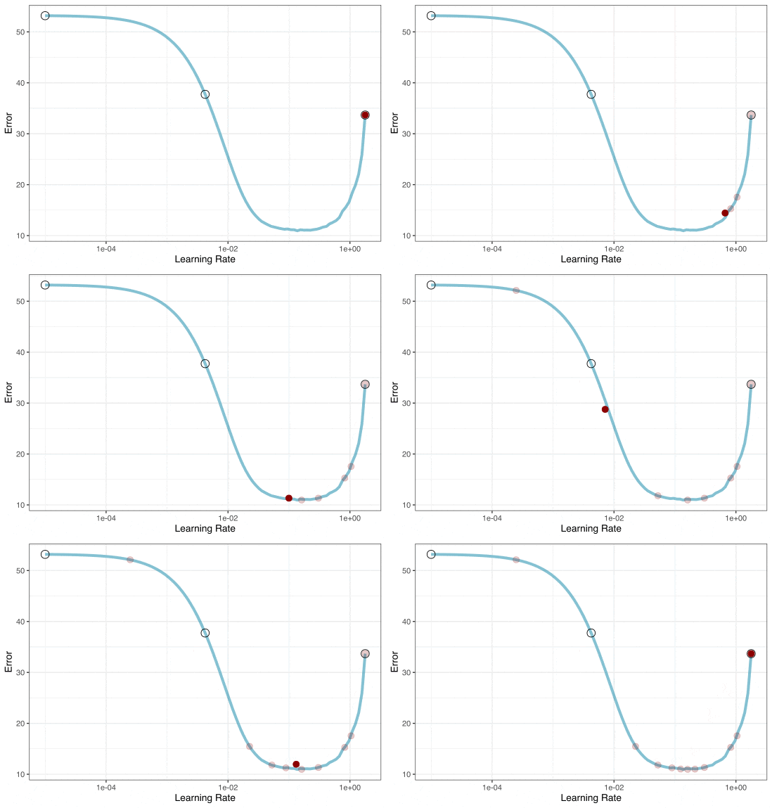
Grid Search

Parameters

• The tidymodels framework provides pre-defined information on tuning parameters (such as their type, range, transformations, etc.).

• The extract_parameter_set_dials() function extracts these tuning parameters and the info.

nnet_param <- 
  nnet_wflow |> 
  extract_parameter_set_dials() 
nnet_param  
#> Collection of 5 parameters for tuning
#> 
#>     identifier          type    object
#>   hidden_units  hidden_units nparam[+]
#>        penalty       penalty nparam[+]
#>     activation    activation dparam[+]
#>     learn_rate    learn_rate nparam[+]
#>  class_weights class_weights nparam[+]
#> 

Different types of grids

Space-filling designs (SFD) attempt to cover the parameter space without redundant candidates. We recommend these the most, and they are the default.

Extract and update parameters

nnet_param <- 
  nnet_param |> 
  update(class_weights = class_weights(c(1, 50)))
  
  nnet_param  
#> Collection of 5 parameters for tuning
#> 
#>     identifier          type    object
#>   hidden_units  hidden_units nparam[+]
#>        penalty       penalty nparam[+]
#>     activation    activation dparam[+]
#>     learn_rate    learn_rate nparam[+]
#>  class_weights class_weights nparam[+]
#> 

Grid Search

ctrl <- control_grid(save_pred = TRUE, save_workflow = TRUE)

set.seed(12)
nnet_res <-
  nnet_wflow |>
  tune_grid(
    resamples = sim_rs,
    grid = 25,
    # The options below are not required by default
    param_info = nnet_param, 
    control = ctrl,
    metrics = cls_mtr
  )

✋ maybe don’t run this just yet…

• tune_grid() is representative of tuning function syntax
• similar to fit_resamples()

Running in parallel

• Grid search, combined with resampling, requires fitting a lot of models!

• These models don’t depend on one another and can be run in parallel.

We can use the future or mirai packages to do this:

cores <- parallelly::availableCores(logical = FALSE)

library(future)
plan(multisession, workers = cores)

# Now call `tune_grid()`!

library(mirai)
daemons(cores)

# Now call `tune_grid()`!

Distributing tasks

When only tuning the model:

Running in parallel

Speed-ups are fairly linear up to the number of physical cores (10 here).

Faceted on the expensiveness of preprocessing used.

Running in parallel

We’ll use mirai as our parallel backend for our notes.

Using 10 cores with mirai, time to execute the previous tune_grid() call was reduced from 256s to 45s, a speed-up of 5.7-fold.

The next slide deck (on racing) includes more examples of speed-ups for a different model.

Grid Search

nnet_res 
#> # Tuning results
#> # 10-fold cross-validation using stratification 
#> # A tibble: 10 × 5
#>    splits             id     .metrics           .notes           .predictions
#>    <list>             <chr>  <list>             <list>           <list>      
#>  1 <split [1348/151]> Fold01 <tibble [100 × 9]> <tibble [0 × 4]> <tibble>    
#>  2 <split [1349/150]> Fold02 <tibble [100 × 9]> <tibble [0 × 4]> <tibble>    
#>  3 <split [1349/150]> Fold03 <tibble [100 × 9]> <tibble [0 × 4]> <tibble>    
#>  4 <split [1349/150]> Fold04 <tibble [100 × 9]> <tibble [0 × 4]> <tibble>    
#>  5 <split [1349/150]> Fold05 <tibble [100 × 9]> <tibble [1 × 4]> <tibble>    
#>  6 <split [1349/150]> Fold06 <tibble [100 × 9]> <tibble [1 × 4]> <tibble>    
#>  7 <split [1349/150]> Fold07 <tibble [100 × 9]> <tibble [1 × 4]> <tibble>    
#>  8 <split [1349/150]> Fold08 <tibble [100 × 9]> <tibble [0 × 4]> <tibble>    
#>  9 <split [1350/149]> Fold09 <tibble [100 × 9]> <tibble [0 × 4]> <tibble>    
#> 10 <split [1350/149]> Fold10 <tibble [100 × 9]> <tibble [1 × 4]> <tibble>    
#> 
#> There were issues with some computations:
#> 
#>   - Warning(s) x1: Early stopping occurred at epoch 2 due to numerical overflow of t...
#>   - Warning(s) x1: Early stopping occurred at epoch 3 due to numerical overflow of t...
#>   - Warning(s) x2: Early stopping occurred at epoch 5 due to numerical overflow of t...
#> 
#> Run `show_notes(.Last.tune.result)` for more information.

Grid results

autoplot(nnet_res)

Brier results

autoplot(nnet_res, metric = "brier_class") + 
  facet_grid(. ~ name, scale = "free_x") + 
  lims(y = c(0.04, 0.22)) # no tanh

ROC curve results

autoplot(nnet_res, metric = "roc_auc") + 
  facet_grid(. ~ name, scale = "free_x") + 
  lims(y = c(0.83, 0.97)) # no tanh

Sensitivity/Specificity results

autoplot(nnet_res, metric = c("sensitivity", "specificity"))

Grid results

• tanh activation 👎👎
• As class weight ⬆️:
  • sensitivity ⬆️
  • specificity ⬇️⬇️
  • Brier: ⬆️
  • ROC AUC: 🤷

Choosing Tuning Parameters

Tuning results

collect_metrics(nnet_res) |> 
  relocate(.metric, mean) 
#> # A tibble: 100 × 11
#>    .metric      mean hidden_units    penalty activation learn_rate class_weights
#>    <chr>       <dbl>        <int>      <dbl> <chr>           <dbl>         <dbl>
#>  1 brier_class 0.135            2 0.00000147 elu           0.0962           17.3
#>  2 roc_auc     0.887            2 0.00000147 elu           0.0962           17.3
#>  3 sensitivity 0.875            2 0.00000147 elu           0.0962           17.3
#>  4 specificity 0.778            2 0.00000147 elu           0.0962           17.3
#>  5 brier_class 0.134            4 0.000464   tanhshrink    0.0736           31.6
#>  6 roc_auc     0.924            4 0.000464   tanhshrink    0.0736           31.6
#>  7 sensitivity 0.863            4 0.000464   tanhshrink    0.0736           31.6
#>  8 specificity 0.802            4 0.000464   tanhshrink    0.0736           31.6
#>  9 brier_class 0.203            6 0.00000383 relu          0.00224          41.8
#> 10 roc_auc     0.880            6 0.00000383 relu          0.00224          41.8
#> # ℹ 90 more rows
#> # ℹ 4 more variables: .estimator <chr>, n <int>, std_err <dbl>, .config <chr>

Tuning results

collect_metrics(nnet_res, summarize = FALSE) |> 
  relocate(.metric, .estimate)
#> # A tibble: 1,000 × 10
#>    .metric     .estimate id     hidden_units    penalty activation learn_rate
#>    <chr>           <dbl> <chr>         <int>      <dbl> <chr>           <dbl>
#>  1 sensitivity    1      Fold01            2 0.00000147 elu            0.0962
#>  2 specificity    0.851  Fold01            2 0.00000147 elu            0.0962
#>  3 brier_class    0.0886 Fold01            2 0.00000147 elu            0.0962
#>  4 roc_auc        0.972  Fold01            2 0.00000147 elu            0.0962
#>  5 sensitivity    0.941  Fold02            2 0.00000147 elu            0.0962
#>  6 specificity    0.887  Fold02            2 0.00000147 elu            0.0962
#>  7 brier_class    0.0847 Fold02            2 0.00000147 elu            0.0962
#>  8 roc_auc        0.974  Fold02            2 0.00000147 elu            0.0962
#>  9 sensitivity    0.882  Fold03            2 0.00000147 elu            0.0962
#> 10 specificity    0.872  Fold03            2 0.00000147 elu            0.0962
#> # ℹ 990 more rows
#> # ℹ 3 more variables: class_weights <dbl>, .estimator <chr>, .config <chr>

Choose a parameter combination

show_best(nnet_res, metric = "brier_class") |> 
  relocate(.metric, mean) 
#> # A tibble: 5 × 11
#>   .metric       mean hidden_units   penalty activation  learn_rate class_weights
#>   <chr>        <dbl>        <int>     <dbl> <chr>            <dbl>         <dbl>
#> 1 brier_class 0.0496           36 0.0000261 elu            0.0562           3.04
#> 2 brier_class 0.0705           14 0.000178  tanhshrink     0.0329           1   
#> 3 brier_class 0.0720           18 0.0562    log_sigmoid    0.631           19.4 
#> 4 brier_class 0.0962           40 0.0215    tanh           0.00293          7.12
#> 5 brier_class 0.100            44 0.383     log_sigmoid    0.0430          27.5 
#> # ℹ 4 more variables: .estimator <chr>, n <int>, std_err <dbl>, .config <chr>

Choose a parameter combination

Create your own tibble for final parameters or use one of the tune::select_*() functions:

nnet_best <- select_best(nnet_res, metric = "brier_class")
nnet_best
#> # A tibble: 1 × 6
#>   hidden_units   penalty activation learn_rate class_weights .config         
#>          <int>     <dbl> <chr>           <dbl>         <dbl> <chr>           
#> 1           36 0.0000261 elu            0.0562          3.04 pre0_mod18_post0

collect_metrics(nnet_res) |> 
  inner_join(nnet_best) |> 
  select(.metric, mean)
#> # A tibble: 4 × 2
#>   .metric       mean
#>   <chr>        <dbl>
#> 1 brier_class 0.0496
#> 2 roc_auc     0.965 
#> 3 sensitivity 0.828 
#> 4 specificity 0.950

Checking (Approximate) Calibration

nnet_holdout_pred <-
  nnet_res |> 
  collect_predictions(
    parameters = nnet_best
  )

nnet_holdout_pred |>
  cal_plot_windowed(
    truth = class,
    estimate = .pred_event,
    window_size = 0.2,
    step_size = 0.025,
  )

This plot pools the out-of-sample predictions. Our Brier estimate is the mean of 10 data sets.

The curve is approximate for that reason.

Multiple goals

Optimizing the Brier score optimizes for accuracy and calibration of the class probabilities.

That’s counter-productive to finding the rare class “event” events.

Can we find a way to optimize multiple metrics at once?

There are a few ways, and we’ll focus on desirability functions.

Desirability functions

We create simple functions to translate our variable to [0, 1]; 1.0 is most desirable.

We can combine them with a geometric mean.

Multimetric optimization

show_best_desirability(
  nnet_res, 
  maximize(sensitivity),
  minimize(brier_class),
  constrain(specificity, low = 0.8, high = 1.0)
) |> 
  relocate(class_weights, sensitivity, specificity, brier_class, .d_overall) 
#> # A tibble: 5 × 14
#>   class_weights sensitivity specificity brier_class .d_overall hidden_units
#>           <dbl>       <dbl>       <dbl>       <dbl>      <dbl>        <int>
#> 1          48.0       0.947       0.811      0.127       0.926           34
#> 2          33.7       0.941       0.805      0.130       0.919           32
#> 3          25.5       0.899       0.850      0.101       0.918           28
#> 4          29.6       0.917       0.830      0.117       0.915           38
#> 5          19.4       0.852       0.914      0.0720      0.907           18
#> # ℹ 8 more variables: penalty <dbl>, activation <chr>, learn_rate <dbl>,
#> #   .config <chr>, roc_auc <dbl>, .d_max_sensitivity <dbl>,
#> #   .d_min_brier_class <dbl>, .d_box_specificity <dbl>

However…

more_sens <-
  select_best_desirability(
    nnet_res,
    maximize(sensitivity),
    minimize(brier_class),
    constrain(specificity, low = 0.8, high = 1.0)
  )

nnet_res |>
  collect_predictions(
    parameters = more_sens
  ) |>
  cal_plot_windowed(
    truth = class,
    estimate = .pred_event,
    window_size = 0.2,
    step_size = 0.025,
  )

The curve hugging the bottom of the plot means that we are drastically overestimating the probability of the “event” class relative to how often it occurs “in the wild.”

That’s the point of cost-sensitive learning, but it’s bad for calibration.

Conflicting goals

The problem here is that we are biasing the probability estimates so that we can predict more data to be the rare “event” class using a default probability cutoff of 1/2.

That is compromising the overall model fit; our probabilities are not accurate.

• If we don’t use the class probability estimates, this is fine.

In the postprocessing slides, we’ll examine an alternative approach that involves different kinds of tradeoffs.

Fitting a workflow

Let’s say that we want to train the model on the “best” parameter estimates.

We can use a tibble of tuning parameters and splice them into the workflow in place of tune():

set.seed(398)
nnet_sens_fit <-
  nnet_wflow |>
  finalize_workflow(more_sens) |>
  fit(sim_train)

nnet_sens_fit |> extract_fit_engine()
#> Multilayer perceptron
#> 
#> relu activation,
#> 34 hidden units,
#> 1,124 model parameters
#> 1,499 samples, 30 features, 2 classes 
#> class weights event=47.95833, no_event= 1.00000 
#> weight decay: 6.812921e-10 
#> dropout proportion: 0 
#> batch size: 1350 
#> learn rate: 0.006556418 
#> validation loss after 13 epochs: 0.0969

Ordering off of the menu

If we want to choose from the numerically best for an existing metric, there is a simpler function:

set.seed(398)
mlp_brier_fit <-
  nnet_res |>
  fit_best(metric = "brier_class")

mlp_brier_fit |> extract_fit_engine()
#> Multilayer perceptron
#> 
#> elu activation,
#> 36 hidden units,
#> 1,190 model parameters
#> 1,499 samples, 30 features, 2 classes 
#> class weights event=3.041667, no_event=1.000000 
#> weight decay: 2.610157e-05 
#> dropout proportion: 0 
#> batch size: 1350 
#> learn rate: 0.05623413 
#> validation loss after 2 epochs: 0.304

Extracting Results

If we want to know about the resampled workflow, we can write a function that can return information from tune_grid().

For example, this one can save the optimization process results:

extract_iter_hist <- function(wflow) {
  require(tidymodels)
  require(tibble)
  wflow |>
    extract_fit_engine() |>
    pluck("loss") |>
    as_tibble_col("loss") |>
    mutate(epoch = row_number() - 1)
}

mlp_brier_fit |> 
  extract_iter_hist() |> 
  slice(1:5)
#> # A tibble: 5 × 2
#>    loss epoch
#>   <dbl> <dbl>
#> 1 0.696     0
#> 2 0.304     1
#> 3 0.217     2
#> 4 0.316     3
#> 5 0.619     4

Your turn

1. Read the docs for control_grid(), specifically the extract option.
2. Create a control object that extracts the iteration history.
3. Re-run tune_grid() with the same grid (or fewer grid points) and use the control option with the extraction function.
4. Afterward use collect_extracts() to get the results.
5. Plot the iteration history for one or more grid points, coloring by the resample id.

Parallel processing will make this go more quickly.

10:00

What’s next

Let’s look at racing: an old variation of grid search that adaptively processes the grid.

If we are

• initially screening many models/preprocessors/postprocessors and/or
• have a large grid

This can lead to remarkable speed-ups.