5 - Tuning models
Practical Machine Learning with tidymodels
Boosted Trees

Your turn

Open the help page for boost_tree() (via ?boost_tree).
Look at the engine documentation for xgboost models.
Grid search
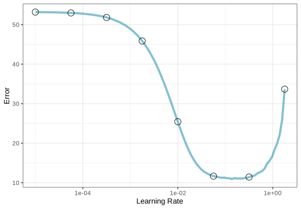
A small grid of points trying to minimize the error via learning rate:

Grid search
In reality, we would probably sample the space more densely:
Iterative Search
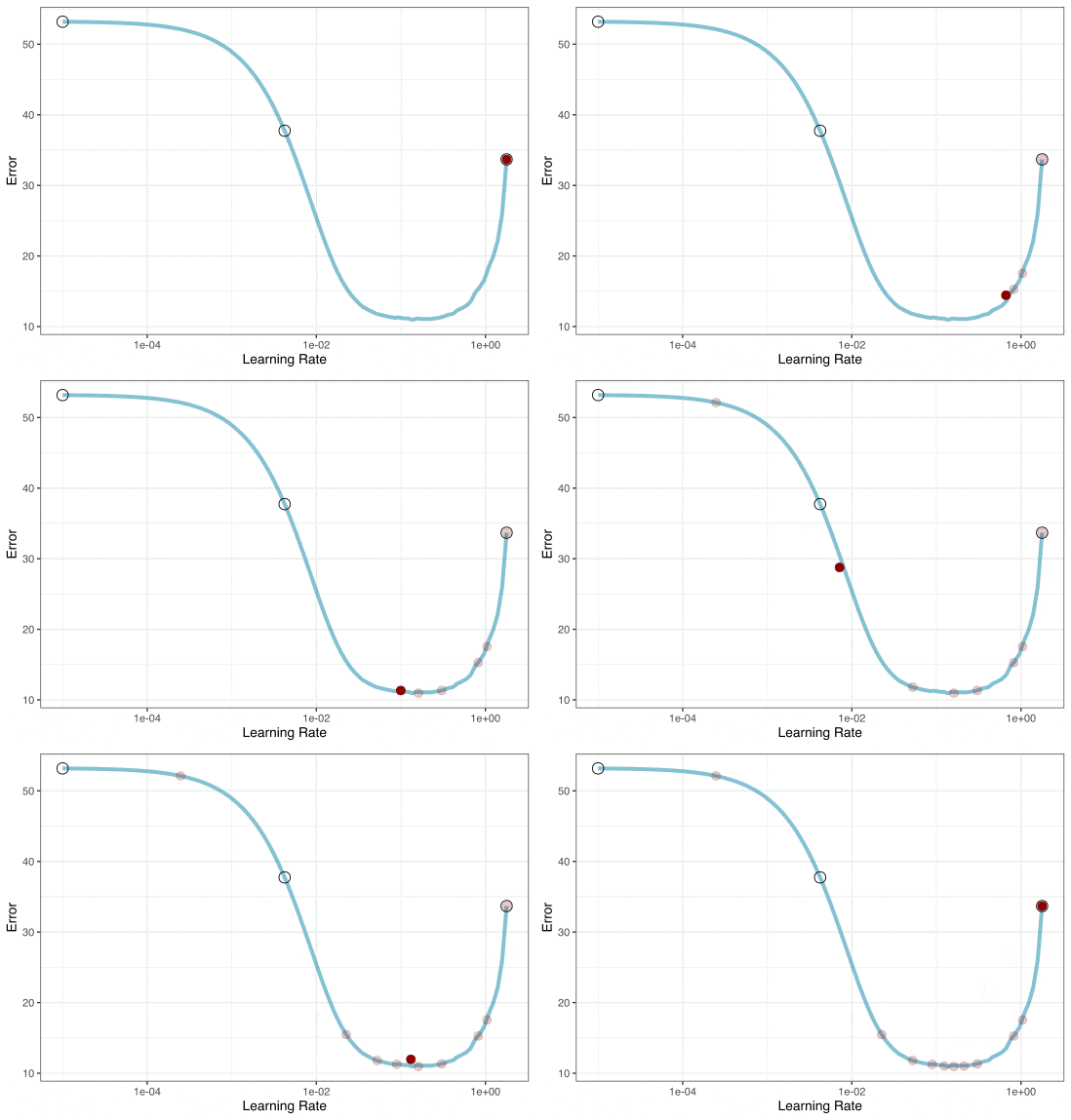
We could start with a few points and search the space:
Different types of grids ![]()


Space-filling designs (SFD) attempt to cover the parameter space without redundant candidates. We recommend these the most, and they are the default.
Compare results
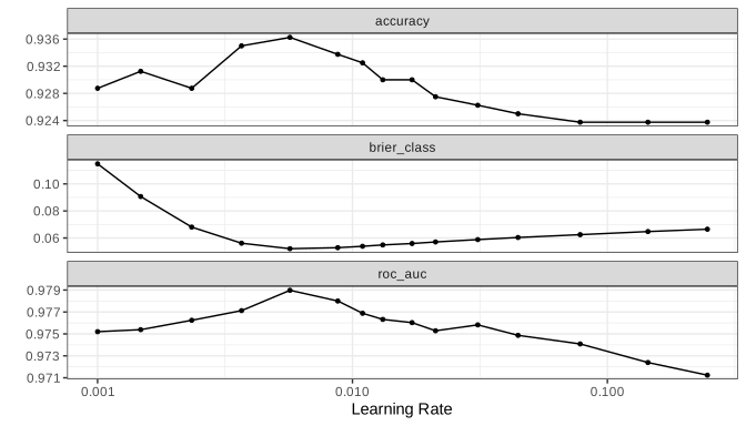
Inspecting results and selecting the best-performing hyperparameter(s):
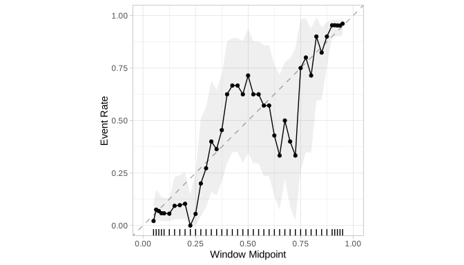
Checking (Approximate) Calibration ![]()
![]()


Distributing tasks
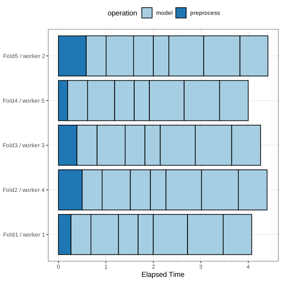
When only tuning the model:
Running in parallel
Speed-ups are fairly linear up to the number of physical cores (10 here).

Your turn
Modify your model workflow to tune additional parameters.
Use grid search to find the best parameter(s).
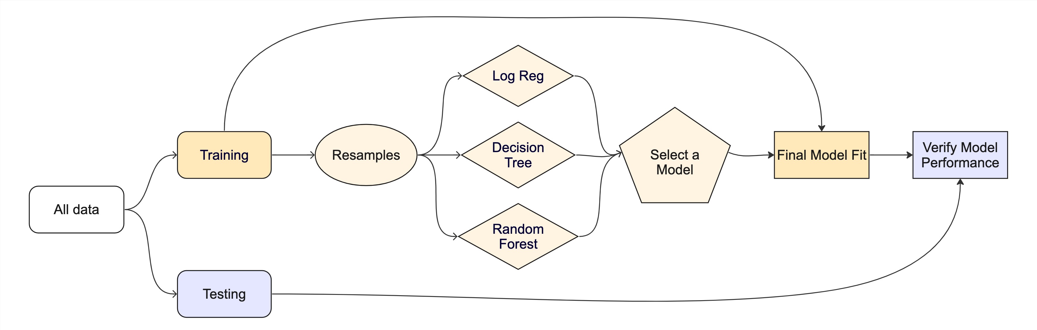
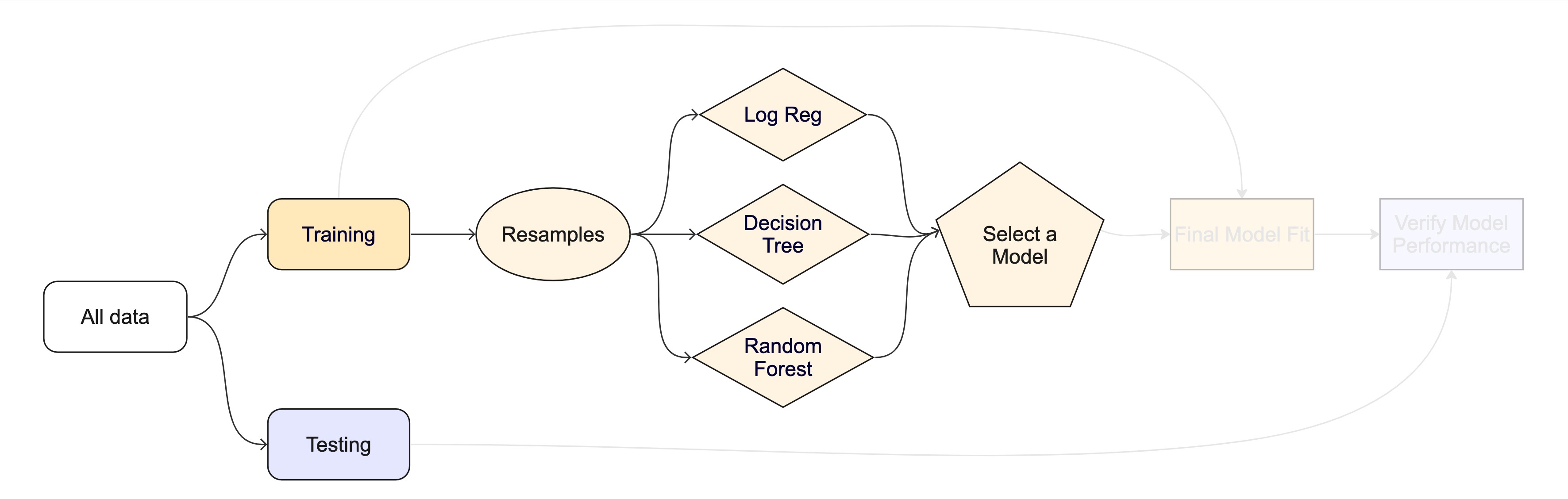
The whole game - status update
The final fit ![]()
Suppose that we are happy with our boosted tree model.
Let’s fit the model on the training set and verify our performance using the test set.
We’ve shown you fit() and predict() (+ augment()) but there is a shortcut:
bst_final_wflow <- finalize_workflow(bst_wflow, best_parameter)
# cls_split has train + test info
set.seed(690)
final_res <- last_fit(bst_final_wflow, cls_split)

final_res
#> # Resampling results
#> # Manual resampling
#> # A tibble: 1 × 6
#>   splits            id               .metrics .notes   .predictions .workflow
#>   <list>            <chr>            <list>   <list>   <list>       <list>
#> 1 <split [800/200]> train/test split <tibble> <tibble> <tibble>     <workflow>
What is in final_res? ![]()
These are metrics computed with the test set
What is in final_res? ![]()
collect_predictions(final_res)
#> # A tibble: 200 × 7
#>    .pred_class .pred_class_1 .pred_class_2 id               class   .row .config
#>    <fct>               <dbl>         <dbl> <chr>            <fct>  <int> <chr>
#>  1 class_1            0.977         0.0233 train/test split class…     1 pre0_m…
#>  2 class_2            0.164         0.836  train/test split class…     3 pre0_m…
#>  3 class_1            0.977         0.0233 train/test split class…     7 pre0_m…
#>  4 class_1            0.977         0.0233 train/test split class…     9 pre0_m…
#>  5 class_2            0.0460        0.954  train/test split class…    12 pre0_m…
#>  6 class_1            0.924         0.0760 train/test split class…    22 pre0_m…
#>  7 class_2            0.0460        0.954  train/test split class…    25 pre0_m…
#>  8 class_1            0.530         0.470  train/test split class…    27 pre0_m…
#>  9 class_1            0.977         0.0233 train/test split class…    28 pre0_m…
#> 10 class_1            0.977         0.0233 train/test split class…    32 pre0_m…
#> # ℹ 190 more rows
What is in final_res? ![]()
![]()
What is in final_res? ![]()
extract_workflow(final_res)
#> ══ Workflow [trained] ════════════════════════════════════════════════
#> Preprocessor: Formula
#> Model: boost_tree()
#>
#> ── Preprocessor ──────────────────────────────────────────────────────
#> class ~ .
#>
#> ── Model ─────────────────────────────────────────────────────────────
#> ##### xgb.Booster
#> call:
#>   xgboost::xgb.train(params = list(eta = 0.0056848552336798, max_depth = 6,
#>     gamma = 0, colsample_bytree = 1, colsample_bynode = 1, min_child_weight = 1,
#>     subsample = 1, nthread = 1, objective = "binary:logistic"),
#>     data = x$data, nrounds = 500, evals = x$watchlist, verbose = 0)
#> # of features: 2
#> # of rounds:  500
#> callbacks:
#>    evaluation_log
#> evaluation_log:
#>   iter training_logloss
#>  <num>            <num>
#>      1        0.6313728
#>      2        0.6268702
#>    ---              ---
#>    499        0.1109659
#>    500        0.1107976
Use this for prediction on new data, like for deploying
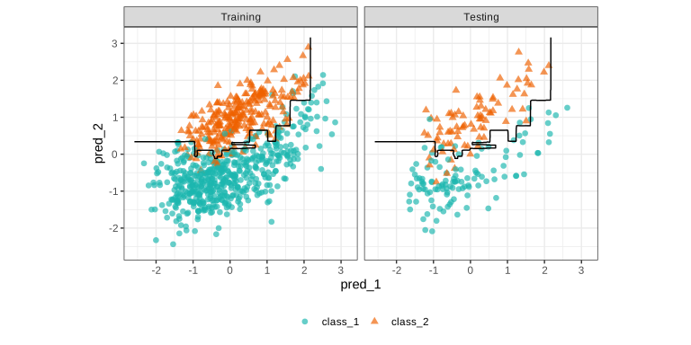
Class Boundary
The whole game