library(tidymodels)

set.seed(123)
cls_split <- initial_split(cls_data_2026, prop = 0.8)
cls_train <- training(cls_split)
cls_test <- testing(cls_split)

tree_spec <- decision_tree(cost_complexity = 0.0001, mode = "classification")
cls_wflow <- workflow(class ~ ., tree_spec)
cls_fit <- fit(cls_wflow, cls_train)4 - Evaluating models
Practical Machine Learning with tidymodels
Confusion matrix ![]()

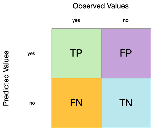
Confusion matrix ![]()
Confusion matrix ![]()

Metrics for model performance ![]()
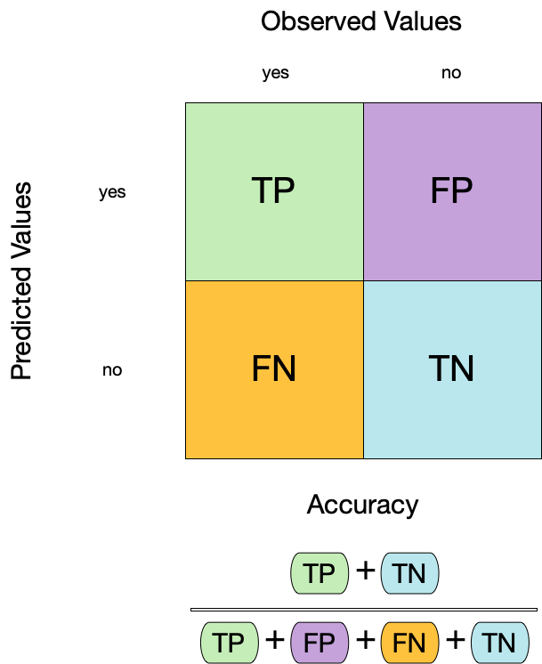
Dangers of accuracy ![]()
We need to be careful of using accuracy() since it can give “good” performance by only predicting one way with imbalanced data:
Separation and calibration
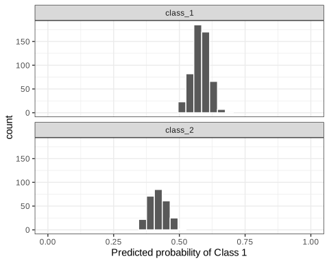
Accuracy measures separation.
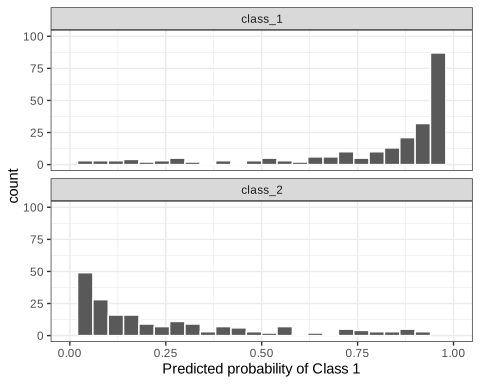
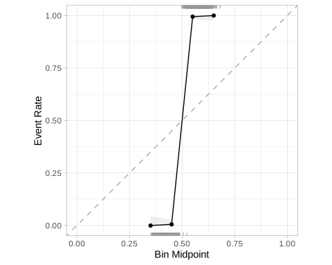
The Brier score captures calibration.
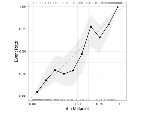
Separation and (bad) calibration
Excellent separation
Terrible calibration.
Your turn

The probably package was used to make the calibration plots:
Try the other calibration curve methods in probably:
Do you prefer one over the others?
Metrics for model performance ![]()
We can use metric_set() to combine multiple calculations into one
Metrics for model performance ![]()
Metrics and metric sets work with grouped data frames!
lr_re_pred |>
  mutate(group = rep_len(LETTERS[1:3], nrow(cls_train))) |>
  group_by(group) |>
  cls_metrics(truth = class, estimate = .pred_class, .pred_class_1)
#> # A tibble: 6 × 4
#>   group .metric     .estimator .estimate
#>   <chr> <chr>       <chr>          <dbl>
#> 1 A     accuracy    binary        0.899
#> 2 B     accuracy    binary        0.906
#> 3 C     accuracy    binary        0.932
#> 4 A     brier_class binary        0.0689
#> 5 B     brier_class binary        0.0693
#> 6 C brier_class binary 0.0613Dangers of overfitting
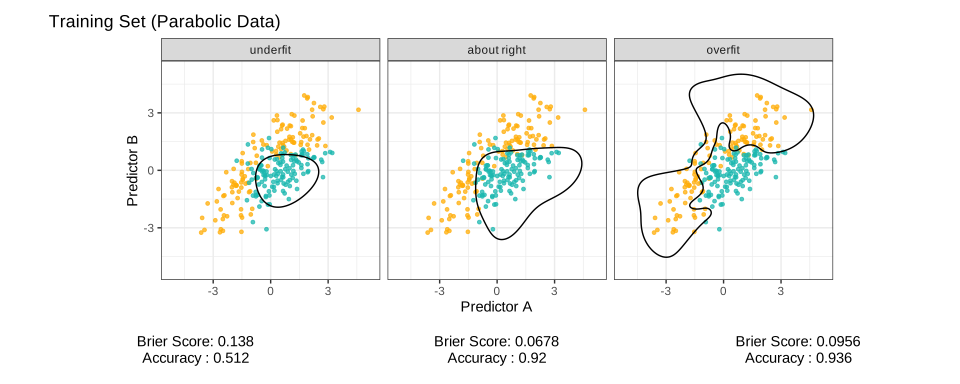
Dangers of overfitting ⚠️
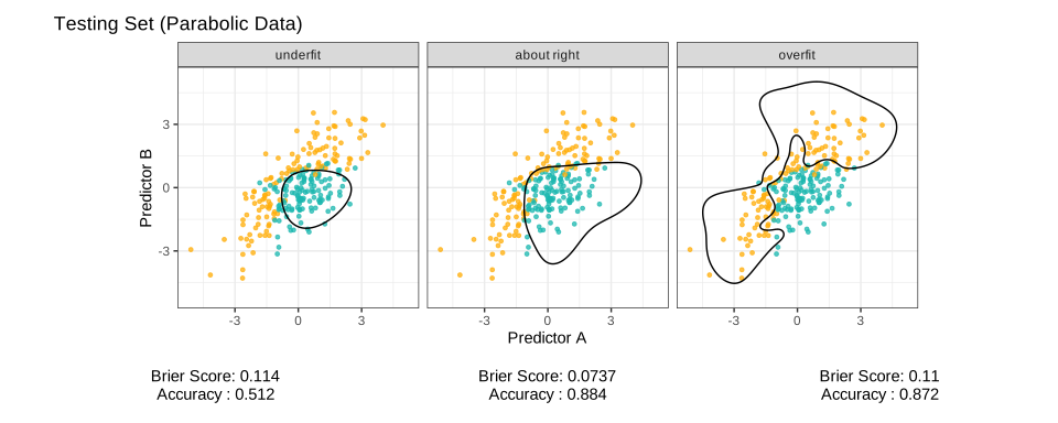
Dangers of overfitting ⚠️ ![]()
lr_fit |>
  augment(cls_train) |>
  print(n = 5)
#> # A tibble: 800 × 6
#>   .pred_class .pred_class_1 .pred_class_2  pred_1 pred_2 class
#>   <fct>               <dbl>         <dbl>   <dbl>  <dbl> <fct>
#> 1 class_1            0.832       0.168    -1.35   -0.446 class_1
#> 2 class_1            0.892       0.108    -0.354  -0.181 class_1
#> 3 class_2            0.0434      0.957     0.105   1.12  class_2
#> 4 class_1            0.999       0.000548  0.0203 -1.20  class_1
#> 5 class_1            0.963       0.0373   -0.831  -0.607 class_1
#> # ℹ 795 more rows
We call this “resubstitution” or “repredicting the training set”
Dangers of overfitting ⚠️ ![]()
We call this a “resubstitution estimate”
Dangers of overfitting ⚠️ ![]()
Dangers of overfitting ⚠️ ![]()
Why aren’t the numbers very different?
Can basic logistic regression overfit?
⚠️ Remember that we’re demonstrating overfitting
⚠️ Don’t use the test set until the end of your modeling analysis
Dangers of overfitting ⚠️ ![]()
What if we want to compare more models?
And/or more model configurations?
And we want to understand if these are important differences?
Cross-validation
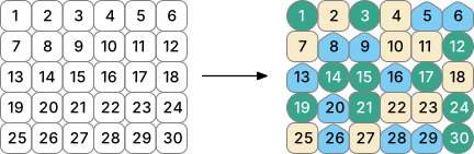
Cross-validation
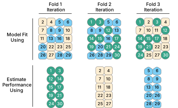
Your turn
If we use 10 folds, what percent of the training data
- ends up in analysis
- ends up in assessment
Cross-validation ![]()

vfold_cv(cls_train) # v = 10 is default
#> #  10-fold cross-validation
#> # A tibble: 10 × 2
#>    splits           id
#>    <list>           <chr>
#>  1 <split [720/80]> Fold01
#>  2 <split [720/80]> Fold02
#>  3 <split [720/80]> Fold03
#>  4 <split [720/80]> Fold04
#>  5 <split [720/80]> Fold05
#>  6 <split [720/80]> Fold06
#>  7 <split [720/80]> Fold07
#>  8 <split [720/80]> Fold08
#>  9 <split [720/80]> Fold09
#> 10 <split [720/80]> Fold10
Cross-validation ![]()
What is in this?
Cross-validation ![]()
Cross-validation ![]()
We’ll use this setup:
set.seed(343)
cls_folds <- vfold_cv(cls_train, v = 10)
cls_folds
#> #  10-fold cross-validation
#> # A tibble: 10 × 2
#>    splits           id
#>    <list>           <chr>
#>  1 <split [720/80]> Fold01
#>  2 <split [720/80]> Fold02
#>  3 <split [720/80]> Fold03
#>  4 <split [720/80]> Fold04
#>  5 <split [720/80]> Fold05
#>  6 <split [720/80]> Fold06
#>  7 <split [720/80]> Fold07
#>  8 <split [720/80]> Fold08
#>  9 <split [720/80]> Fold09
#> 10 <split [720/80]> Fold10
Set the seed when creating resamples
Evaluating model performance ![]()

We can reliably measure performance using only the training data 🎉
Comparing metrics ![]()
How do the metrics from resampling compare to the metrics from training and testing?
The Brier score previously was
- 0.067 for the training set
- 0.074 for test set
Remember that:
⚠️ the training set gives you overly optimistic metrics
⚠️ the test set is precious
Your turn
Rerun the same code three times with different random number seeds.
How much do the results change?
Evaluating model performance ![]()
# Save the assessment set results
ctrl_rs <- control_resamples(save_pred = TRUE)
cls_res <- fit_resamples(lr_wflow, cls_folds, control = ctrl_rs)

cls_res
#> # Resampling results
#> # 10-fold cross-validation
#> # A tibble: 10 × 5
#>    splits           id     .metrics         .notes           .predictions
#>    <list>           <chr>  <list>           <list>           <list>
#>  1 <split [720/80]> Fold01 <tibble [3 × 4]> <tibble [0 × 4]> <tibble [80 × 6]>
#>  2 <split [720/80]> Fold02 <tibble [3 × 4]> <tibble [0 × 4]> <tibble [80 × 6]>
#>  3 <split [720/80]> Fold03 <tibble [3 × 4]> <tibble [0 × 4]> <tibble [80 × 6]>
#>  4 <split [720/80]> Fold04 <tibble [3 × 4]> <tibble [0 × 4]> <tibble [80 × 6]>
#>  5 <split [720/80]> Fold05 <tibble [3 × 4]> <tibble [0 × 4]> <tibble [80 × 6]>
#>  6 <split [720/80]> Fold06 <tibble [3 × 4]> <tibble [0 × 4]> <tibble [80 × 6]>
#>  7 <split [720/80]> Fold07 <tibble [3 × 4]> <tibble [0 × 4]> <tibble [80 × 6]>
#>  8 <split [720/80]> Fold08 <tibble [3 × 4]> <tibble [0 × 4]> <tibble [80 × 6]>
#>  9 <split [720/80]> Fold09 <tibble [3 × 4]> <tibble [0 × 4]> <tibble [80 × 6]>
#> 10 <split [720/80]> Fold10 <tibble [3 × 4]> <tibble [0 × 4]> <tibble [80 × 6]>
Evaluating model performance ![]()
![]()

probably has a nice interface for calibration curves:
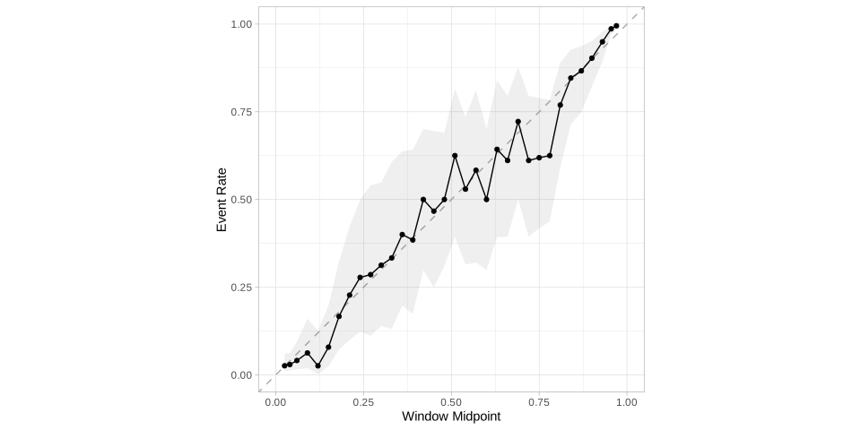
The out-of-sample predictions are pooled before computing the calibration curve.
Evaluating model performance ![]()
# Save the assessment set results
cls_preds <- collect_predictions(cls_res)

cls_preds |> slice(1:5)
#> # A tibble: 5 × 7
#>   .pred_class .pred_class_1 .pred_class_2 id     class    .row .config
#>   <fct>               <dbl>         <dbl> <chr>  <fct>   <int> <chr>
#> 1 class_1             1.000      0.000371 Fold01 class_1    14 pre0_mod0_post0
#> 2 class_2             0.267      0.733    Fold01 class_1    24 pre0_mod0_post0
#> 3 class_1             0.997      0.00253  Fold01 class_1    32 pre0_mod0_post0
#> 4 class_1             0.748      0.252    Fold01 class_1    41 pre0_mod0_post0
#> 5 class_1             1.000      0.000323 Fold01 class_1    42 pre0_mod0_post0
Evaluating model performance ![]()
cls_preds |>
  group_by(id) |>
  cls_metrics(truth = class, estimate = .pred_class, .pred_class_1)
#> # A tibble: 20 × 4
#>    id     .metric     .estimator .estimate
#>    <chr>  <chr>       <chr>          <dbl>
#>  1 Fold01 accuracy    binary        0.862
#>  2 Fold02 accuracy    binary        0.85
#>  3 Fold03 accuracy    binary        0.988
#>  4 Fold04 accuracy    binary        0.925
#>  5 Fold05 accuracy    binary        0.888
#>  6 Fold06 accuracy    binary        0.925
#>  7 Fold07 accuracy    binary        0.925
#>  8 Fold08 accuracy    binary        0.938
#>  9 Fold09 accuracy    binary        0.912
#> 10 Fold10 accuracy    binary        0.9
#> 11 Fold01 brier_class binary        0.0891
#> 12 Fold02 brier_class binary        0.0908
#> 13 Fold03 brier_class binary        0.0245
#> 14 Fold04 brier_class binary        0.0647
#> 15 Fold05 brier_class binary        0.0974
#> 16 Fold06 brier_class binary        0.0588
#> 17 Fold07 brier_class binary        0.0573
#> 18 Fold08 brier_class binary        0.0659
#> 19 Fold09 brier_class binary        0.0634
#> 20 Fold10 brier_class binary        0.0678
Where are the fitted models? ![]()
cls_res
#> # Resampling results
#> # 10-fold cross-validation
#> # A tibble: 10 × 5
#>    splits           id     .metrics         .notes           .predictions
#>    <list>           <chr>  <list>           <list>           <list>
#>  1 <split [720/80]> Fold01 <tibble [3 × 4]> <tibble [0 × 4]> <tibble [80 × 6]>
#>  2 <split [720/80]> Fold02 <tibble [3 × 4]> <tibble [0 × 4]> <tibble [80 × 6]>
#>  3 <split [720/80]> Fold03 <tibble [3 × 4]> <tibble [0 × 4]> <tibble [80 × 6]>
#>  4 <split [720/80]> Fold04 <tibble [3 × 4]> <tibble [0 × 4]> <tibble [80 × 6]>
#>  5 <split [720/80]> Fold05 <tibble [3 × 4]> <tibble [0 × 4]> <tibble [80 × 6]>
#>  6 <split [720/80]> Fold06 <tibble [3 × 4]> <tibble [0 × 4]> <tibble [80 × 6]>
#>  7 <split [720/80]> Fold07 <tibble [3 × 4]> <tibble [0 × 4]> <tibble [80 × 6]>
#>  8 <split [720/80]> Fold08 <tibble [3 × 4]> <tibble [0 × 4]> <tibble [80 × 6]>
#>  9 <split [720/80]> Fold09 <tibble [3 × 4]> <tibble [0 × 4]> <tibble [80 × 6]>
#> 10 <split [720/80]> Fold10 <tibble [3 × 4]> <tibble [0 × 4]> <tibble [80 × 6]>
🗑️
The whole game - status update
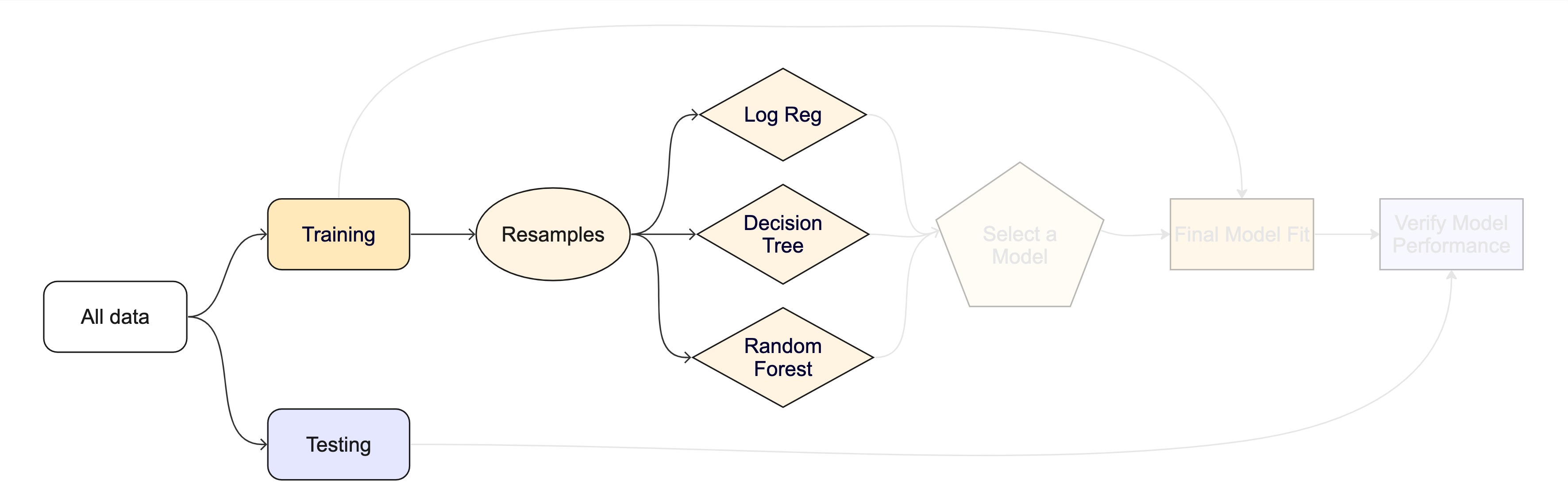
Metrics for model performance ![]()
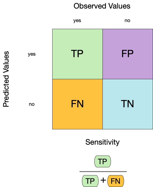
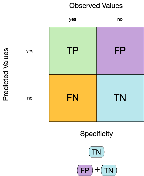
Metrics for model performance ![]()
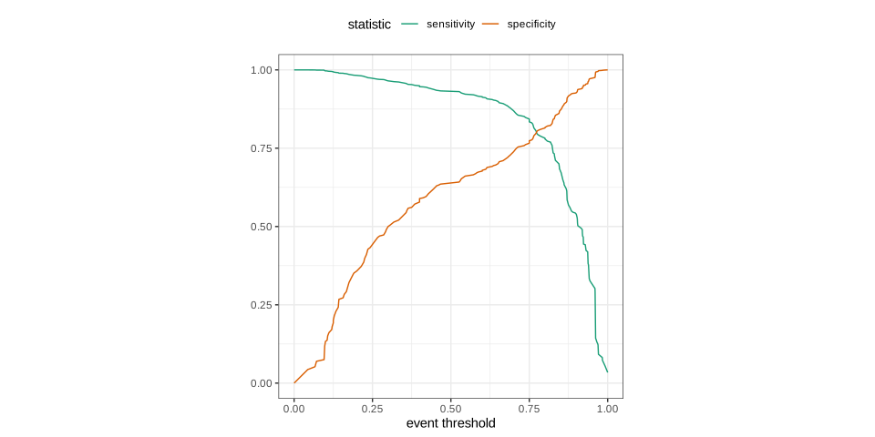
Varying the threshold
ROC curves
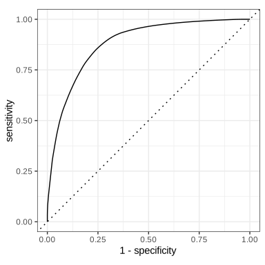
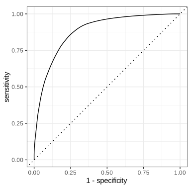
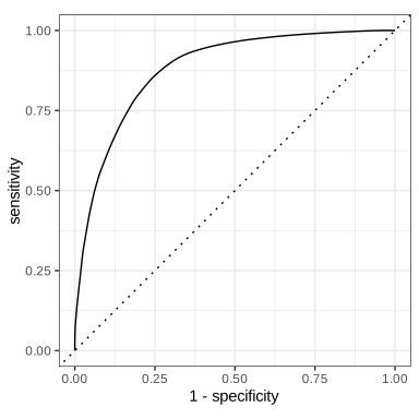
For an ROC (receiver operator characteristic) curve, we plot
- the false positive rate (1 - specificity) on the x-axis
- the true positive rate (sensitivity) on the y-axis
with sensitivity and specificity calculated at all possible thresholds.
ROC curves
We can use the area under the ROC curve as a classification metric:
- ROC AUC = 1 💯
- ROC AUC = 1/2 😢
ROC curves ![]()
# Assumes _first_ factor level is event; there are options to change that
lr_re_pred |>
  roc_curve(truth = class, .pred_class_1) |>
  slice(1, 20, 50)
#> # A tibble: 3 × 3
#>   .threshold specificity sensitivity
#>        <dbl>       <dbl>       <dbl>
#> 1 -Inf            0            1
#> 2    0.00619      0.0677       1
#> 3    0.0154       0.177        0.998

lr_re_pred |>
  roc_auc(truth = class, .pred_class_1)
#> # A tibble: 1 × 3
#>   .metric .estimator .estimate
#>   <chr>   <chr>          <dbl>
#> 1 roc_auc binary         0.968
ROC curve plot ![]()
Your turn
Compute and plot an ROC curve for your current model.
What data are being used for this ROC curve plot?
Bootstrapping ![]()
set.seed(3214)
bootstraps(cls_train)
#> # Bootstrap sampling
#> # A tibble: 25 × 2
#>    splits            id
#>    <list>            <chr>
#>  1 <split [800/287]> Bootstrap01
#>  2 <split [800/294]> Bootstrap02
#>  3 <split [800/292]> Bootstrap03
#>  4 <split [800/293]> Bootstrap04
#>  5 <split [800/279]> Bootstrap05
#>  6 <split [800/287]> Bootstrap06
#>  7 <split [800/297]> Bootstrap07
#>  8 <split [800/291]> Bootstrap08
#>  9 <split [800/307]> Bootstrap09
#> 10 <split [800/296]> Bootstrap10
#> # ℹ 15 more rows
Your turn
Create:
- Monte Carlo Cross-Validation sets
- validation set
(use the reference guide to find the functions)
Don’t forget to set a seed when you resample!
Monte Carlo Cross-Validation ![]()
set.seed(322)
mc_cv(cls_train, times = 10)
#> # Monte Carlo cross-validation (0.75/0.25) with 10 resamples
#> # A tibble: 10 × 2
#>    splits            id
#>    <list>            <chr>
#>  1 <split [600/200]> Resample01
#>  2 <split [600/200]> Resample02
#>  3 <split [600/200]> Resample03
#>  4 <split [600/200]> Resample04
#>  5 <split [600/200]> Resample05
#>  6 <split [600/200]> Resample06
#>  7 <split [600/200]> Resample07
#>  8 <split [600/200]> Resample08
#>  9 <split [600/200]> Resample09
#> 10 <split [600/200]> Resample10
Validation set ![]()
A validation set is just another type of resample