2 - Your data budget

Practical Machine Learning with tidymodels

A classification data set

We’ve created an simulated data set (based on real data) that has

  • Two numeric predictors (pred_1 and pred_2)
  • A factor column (class) with levels "class_1" and "class_1"
library(tidymodels)
# cls_data_2026 is already loaded from the modeldata package
glimpse(cls_data_2026)
#> Rows: 1,000
#> Columns: 3
#> $ pred_1 <dbl> 0.4304422, -1.2983697, 1.1479129, 1.7931431, -0.8016918, 1.1603…
#> $ pred_2 <dbl> -0.7325339, -0.9398467, 1.6149989, 1.2296319, 0.4030618, 1.5732…
#> $ class  <fct> class_1, class_1, class_2, class_1, class_2, class_2, class_1, …

Your turn

Let’s take 5 minutes and look at the data.

Checklist for predictors

  • Is it ethical to use this variable? (Or even legal?)

  • Will this variable be available at prediction time?

  • Do we think that they are informative?

Data splitting and spending

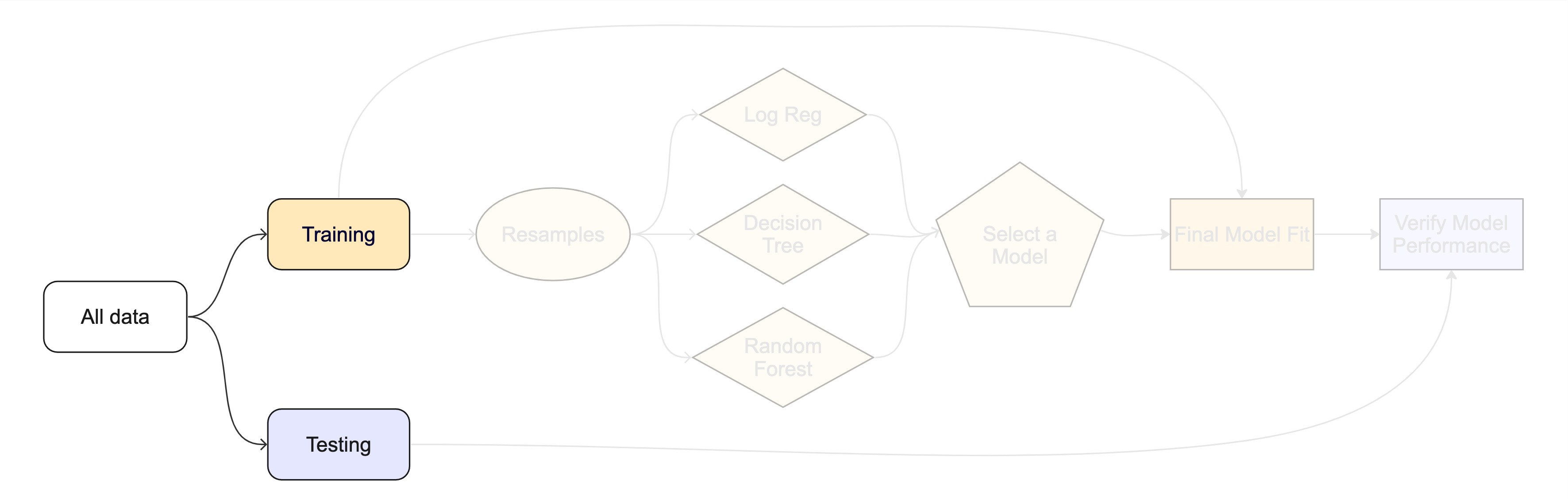
For machine learning, we typically split data into training and test sets:

  • The training set is used to estimate model parameters.
  • The test set is used to find an independent assessment of model performance.

Do not 🚫 use the test set during training.

Data splitting and spending

The more data
we spend 🤑

the better estimates
we’ll get.

Data splitting and spending

  • Spending too much data in training prevents us from computing a good assessment of predictive performance.
  • Spending too much data in testing prevents us from computing a good estimate of model parameters.

Your turn

When is a good time to split your data?

The testing data is precious 💎

The initial split

set.seed(123)
cls_split <- initial_split(cls_data_2026)
cls_split
#> <Training/Testing/Total>
#> <750/250/1000>

What is set.seed()?

To create that split of the data, R generates “pseudo-random” numbers: while they are made to behave like random numbers, their generation is deterministic given a “seed”.

This allows us to reproduce results by setting that seed.

Which seed you pick doesn’t matter, as long as you don’t try a bunch of seeds and pick the one that gives you the best performance.

Accessing the data

cls_train <- training(cls_split)
cls_test <- testing(cls_split)

The training set

cls_train
#> # A tibble: 750 × 3
#>     pred_1  pred_2 class  
#>      <dbl>   <dbl> <fct>  
#>  1 -1.35   -0.446  class_1
#>  2 -0.354  -0.181  class_1
#>  3  0.105   1.12   class_2
#>  4  0.0203 -1.20   class_1
#>  5 -0.831  -0.607  class_1
#>  6  0.150   0.904  class_2
#>  7  0.441  -0.642  class_1
#>  8  1.56   -0.0182 class_1
#>  9  0.200  -0.898  class_1
#> 10 -0.0455 -0.478  class_1
#> # ℹ 740 more rows

The test set

🙈

There are 250 rows and 3 columns in the test set.

Your turn

Split your data so 20% is held out for the test set.

Try out different values in set.seed() to see how the results change.


We recommend using the .qmd files in the classwork/ folder for code exercises. They set you up with the code from the slides.

Data splitting and spending

set.seed(123)
cls_split <- initial_split(cls_data_2026, prop = 0.8)
cls_train <- training(cls_split)
cls_test <- testing(cls_split)

nrow(cls_train)
#> [1] 800
nrow(cls_test)
#> [1] 200

Your turn

Explore the cls_train data on your own!

  • What’s the distribution of the outcome, class?
  • What’s the distribution of numeric variables?

The whole game - status update