3 - Tuning Hyperparameters

Advanced tidymodels

Previously - Setup

library(tidymodels)
library(textrecipes)
library(bonsai)

# Max's usual settings: 
tidymodels_prefer()
theme_set(theme_bw())
options(
  pillar.advice = FALSE, 
  pillar.min_title_chars = Inf
)

reg_metrics <- metric_set(mae, rsq)

data(hotel_rates)
set.seed(295)
hotel_rates <- 
  hotel_rates |> 
  sample_n(5000) |> 
  arrange(arrival_date) |> 
  select(-arrival_date) |> 
  mutate(
    company = factor(as.character(company)),
    country = factor(as.character(country)),
    agent = factor(as.character(agent))
  )

Previously - Data Usage

set.seed(4028)
hotel_split <- initial_split(hotel_rates, strata = avg_price_per_room)

hotel_train <- training(hotel_split)
hotel_test <- testing(hotel_split)

set.seed(472)
hotel_rs <- vfold_cv(hotel_train, strata = avg_price_per_room)

Previously - Feature engineering

library(textrecipes)

hash_rec <-
  recipe(avg_price_per_room ~ ., data = hotel_train) |>
  step_YeoJohnson(lead_time) |>
  # Defaults to 32 signed indicator columns
  step_dummy_hash(agent) |>
  step_dummy_hash(company) |>
  # Regular indicators for the others
  step_dummy(all_nominal_predictors()) |> 
  step_zv(all_predictors())

Optimizing Models via Tuning Parameters

Tuning parameters

Some model or preprocessing parameters cannot be estimated directly from the data.

Some examples:

Tree depth in decision trees
Number of neighbors in a K-nearest neighbor model

Activation function in neural networks?

Sigmoidal functions, ReLu, etc.

Yes, it is a tuning parameter. ✅

Number of feature hashing columns to generate?

Yes, it is a tuning parameter. ✅

Bayesian priors for model parameters?

Hmmmm, probably not. These are based on prior belief. ❌

The random seed?

Nope. It is not. ❌

Optimize tuning parameters

Try different values and measure their performance.

Find good values for these parameters.

Once the value(s) of the parameter(s) are determined, a model can be finalized by fitting the model to the entire training set.

Tagging parameters for tuning

With tidymodels, you can mark the parameters that you want to optimize with a value of tune().

The function itself just returns… itself:

tune()
#> tune()
str(tune())
#>  language tune()

# optionally add a label
tune("I hope that the workshop is going well")
#> tune("I hope that the workshop is going well")

For example…

Optimizing the hash features

Our new recipe is:

hash_rec <-
  recipe(avg_price_per_room ~ ., data = hotel_train) |>
  step_YeoJohnson(lead_time) |>
  step_dummy_hash(agent,   num_terms = tune("agent hash")) |>
  step_dummy_hash(company, num_terms = tune("company hash")) |>
  step_zv(all_predictors())

We will be using a tree-based model in a minute.

The other categorical predictors are left as-is.
That’s why there is no step_dummy().

Boosted Trees

These are popular ensemble methods that build a sequence of tree models.

Each tree uses the results of the previous tree to better predict samples, especially those that have been poorly predicted.

Each tree in the ensemble is saved and new samples are predicted using a weighted average of the votes of each tree in the ensemble.

We’ll focus on the popular lightgbm implementation.

Boosted Tree Tuning Parameters

Some possible parameters:

mtry: The number of predictors randomly sampled at each split (in \([1, ncol(x)]\) or \((0, 1]\)).
trees: The number of trees (\([1, \infty]\), but usually up to thousands)
min_n: The number of samples needed to further split (\([1, n]\)).
learn_rate: The rate that each tree adapts from previous iterations (\((0, \infty]\), usual maximum is 0.1).
stop_iter: The number of iterations of boosting where no improvement was shown before stopping (\([1, trees]\))

Boosted Tree Tuning Parameters

TBH it is usually not difficult to optimize these models.

Often, there are multiple candidate tuning parameter combinations that have very good results.

To demonstrate simple concepts, we’ll look at optimizing the number of trees in the ensemble (between 1 and 100) and the learning rate (\(10^{-5}\) to \(10^{-1}\)).

Boosted Tree Tuning Parameters

We’ll need to load the bonsai package. This has the information needed to use lightgbm

library(bonsai)
lgbm_spec <- 
  boost_tree(trees = tune(), learn_rate = tune()) |> 
  set_mode("regression") |> 
  set_engine("lightgbm", num_threads = 1)

lgbm_wflow <- workflow(hash_rec, lgbm_spec)

Optimize tuning parameters

The main two strategies for optimization are:

Grid search 💠 which tests a pre-defined set of candidate values
Iterative search 🌀 which suggests/estimates new values of candidate parameters to evaluate

Grid search

A small grid of points trying to minimize the error via learning rate:

Grid search

In reality we would probably sample the space more densely:

Iterative Search

We could start with a few points and search the space:

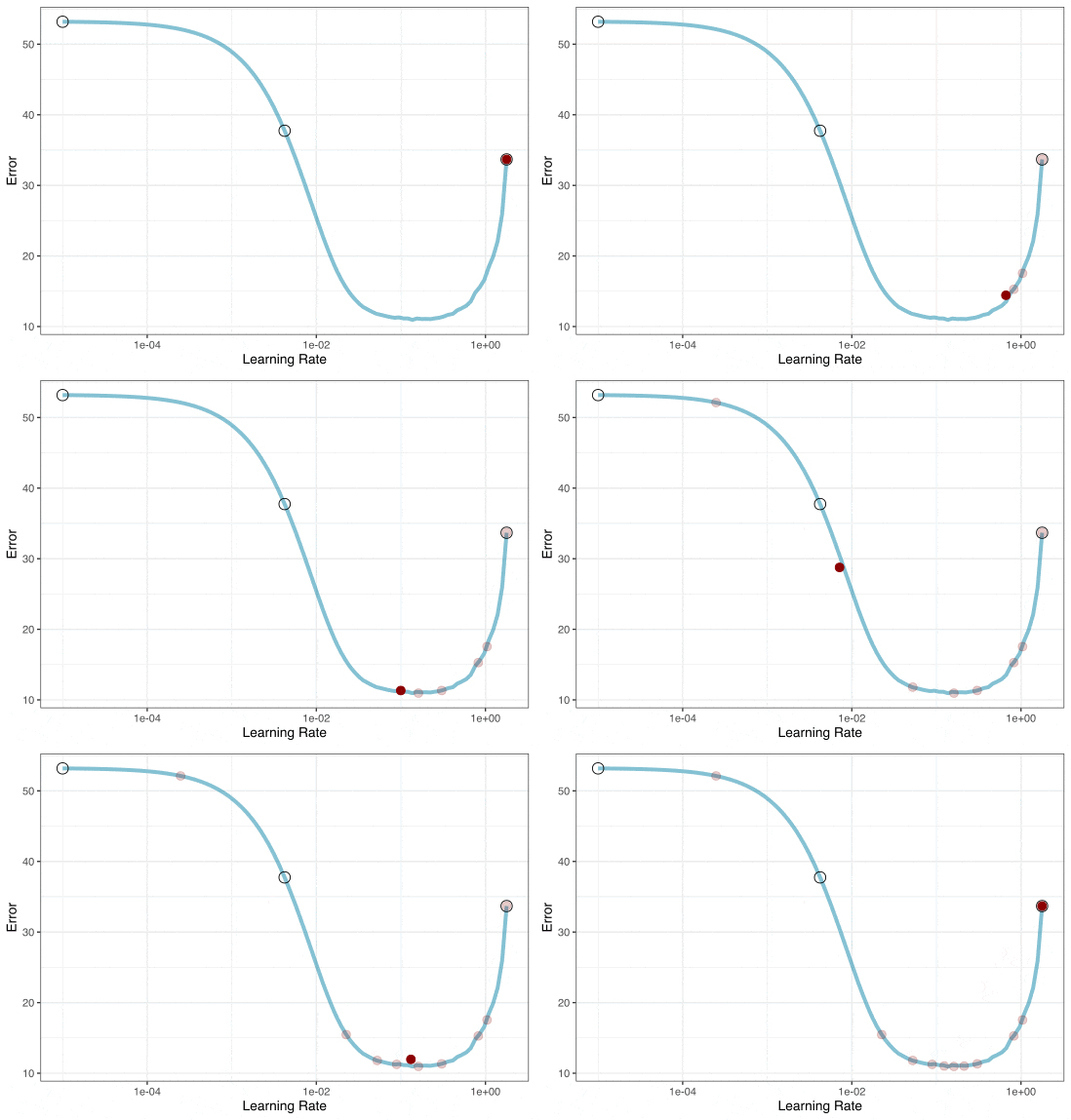
Grid Search

Parameters

The tidymodels framework provides pre-defined information on tuning parameters (such as their type, range, transformations, etc).
The extract_parameter_set_dials() function extracts these tuning parameters and the info.

Grids

Create your grid manually or automatically.
The grid_*() functions can make a grid.

Different types of grids

Space-filling designs (SFD) attempt to cover the parameter space without redundant candidates. We recommend these the most.

Create a grid

lgbm_wflow |> 
  extract_parameter_set_dials()

# Individual functions: 
trees()
learn_rate()

A parameter set can be updated (e.g. to change the ranges).

Create a grid

grid <- 
  lgbm_wflow |> 
  extract_parameter_set_dials() |> 
  grid_space_filling(size = 25)

grid
#> # A tibble: 25 × 4
#>    trees learn_rate `agent hash` `company hash`
#>    <int>      <dbl>        <int>          <int>
#>  1     1   7.50e- 6          574            574
#>  2    84   1.78e- 5         2048           2298
#>  3   167   5.62e-10         1824            912
#>  4   250   4.22e- 5         3250            512
#>  5   334   1.78e- 8          512           2896
#>  6   417   1.33e- 3          322           1625
#>  7   500   1   e- 1         1448           1149
#>  8   584   1   e- 7         1290            256
#>  9   667   2.37e-10          456            724
#> 10   750   1.78e- 2          645            322
#> # ℹ 15 more rows

Your turn

Create a grid for our tunable workflow.

Try creating a regular grid.

03:00

Create a regular grid

grid <- 
  lgbm_wflow |> 
  extract_parameter_set_dials() |> 
  grid_regular(levels = 4)

grid
#> # A tibble: 256 × 4
#>    trees   learn_rate `agent hash` `company hash`
#>    <int>        <dbl>        <int>          <int>
#>  1     1 0.0000000001          256            256
#>  2   667 0.0000000001          256            256
#>  3  1333 0.0000000001          256            256
#>  4  2000 0.0000000001          256            256
#>  5     1 0.0000001             256            256
#>  6   667 0.0000001             256            256
#>  7  1333 0.0000001             256            256
#>  8  2000 0.0000001             256            256
#>  9     1 0.0001                256            256
#> 10   667 0.0001                256            256
#> # ℹ 246 more rows

Your turn

What advantage would a regular grid have?

Update parameter ranges

lgbm_param <- 
  lgbm_wflow |> 
  extract_parameter_set_dials() |> 
  update(trees = trees(c(1L, 100L)),
         learn_rate = learn_rate(c(-5, -1)))

grid <- 
  lgbm_param |> 
  grid_space_filling(size = 25)

grid
#> # A tibble: 25 × 4
#>    trees learn_rate `agent hash` `company hash`
#>    <int>      <dbl>        <int>          <int>
#>  1     1  0.00147            574            574
#>  2     5  0.00215           2048           2298
#>  3     9  0.0000215         1824            912
#>  4    13  0.00316           3250            512
#>  5    17  0.0001             512           2896
#>  6    21  0.0147             322           1625
#>  7    25  0.1               1448           1149
#>  8    29  0.000215          1290            256
#>  9    34  0.0000147          456            724
#> 10    38  0.0464             645            322
#> # ℹ 15 more rows

The results

grid |> 
  ggplot(aes(trees, learn_rate)) +
  geom_point(size = 4) +
  scale_y_log10()

Note that the learning rates are uniform on the log-10 scale and this shows 2 of 4 dimensions.

Use the `tune_*()` functions to tune models

Choosing tuning parameters

Let’s take our previous model and tune more parameters:

lgbm_spec <- 
  boost_tree(trees = tune(), learn_rate = tune(),  min_n = tune()) |> 
  set_mode("regression") |> 
  set_engine("lightgbm", num_threads = 1)

lgbm_wflow <- workflow(hash_rec, lgbm_spec)

# Update the feature hash ranges (log-2 units)
lgbm_param <-
  lgbm_wflow |>
  extract_parameter_set_dials() |>
  update(`agent hash`   = num_hash(c(3, 8)),
         `company hash` = num_hash(c(3, 8)))

Grid Search

set.seed(9)
ctrl <- control_grid(save_pred = TRUE)

lgbm_res <-
  lgbm_wflow |>
  tune_grid(
    resamples = hotel_rs,
    grid = 25,
    # The options below are not required by default
    param_info = lgbm_param, 
    control = ctrl,
    metrics = reg_metrics
  )

Grid Search

lgbm_res 
#> # Tuning results
#> # 10-fold cross-validation using stratification 
#> # A tibble: 10 × 5
#>    splits             id     .metrics          .notes           .predictions        
#>    <list>             <chr>  <list>            <list>           <list>              
#>  1 <split [3372/377]> Fold01 <tibble [50 × 9]> <tibble [0 × 4]> <tibble [9,425 × 9]>
#>  2 <split [3373/376]> Fold02 <tibble [50 × 9]> <tibble [0 × 4]> <tibble [9,400 × 9]>
#>  3 <split [3373/376]> Fold03 <tibble [50 × 9]> <tibble [0 × 4]> <tibble [9,400 × 9]>
#>  4 <split [3373/376]> Fold04 <tibble [50 × 9]> <tibble [0 × 4]> <tibble [9,400 × 9]>
#>  5 <split [3373/376]> Fold05 <tibble [50 × 9]> <tibble [0 × 4]> <tibble [9,400 × 9]>
#>  6 <split [3374/375]> Fold06 <tibble [50 × 9]> <tibble [0 × 4]> <tibble [9,375 × 9]>
#>  7 <split [3375/374]> Fold07 <tibble [50 × 9]> <tibble [0 × 4]> <tibble [9,350 × 9]>
#>  8 <split [3376/373]> Fold08 <tibble [50 × 9]> <tibble [0 × 4]> <tibble [9,325 × 9]>
#>  9 <split [3376/373]> Fold09 <tibble [50 × 9]> <tibble [0 × 4]> <tibble [9,325 × 9]>
#> 10 <split [3376/373]> Fold10 <tibble [50 × 9]> <tibble [0 × 4]> <tibble [9,325 × 9]>

Grid results

autoplot(lgbm_res)

Tuning results

collect_metrics(lgbm_res)
#> # A tibble: 50 × 11
#>    trees min_n    learn_rate `agent hash` `company hash` .metric .estimator   mean     n std_err .config          
#>    <int> <int>         <dbl>        <int>          <int> <chr>   <chr>       <dbl> <int>   <dbl> <chr>            
#>  1  1500    21 0.00000000316            8             60 mae     standard   53.2      10 0.427   pre01_mod19_post0
#>  2  1500    21 0.00000000316            8             60 rsq     standard    0.809    10 0.00661 pre01_mod19_post0
#>  3   917    16 0.0422                   9             39 mae     standard    9.85     10 0.150   pre02_mod12_post0
#>  4   917    16 0.0422                   9             39 rsq     standard    0.946    10 0.00362 pre02_mod12_post0
#>  5   584    13 0.0000001               10             10 mae     standard   53.2      10 0.427   pre03_mod08_post0
#>  6   584    13 0.0000001               10             10 rsq     standard    0.810    10 0.00745 pre03_mod08_post0
#>  7   167    19 0.00000133              12            143 mae     standard   53.2      10 0.426   pre04_mod03_post0
#>  8   167    19 0.00000133              12            143 rsq     standard    0.811    10 0.00698 pre04_mod03_post0
#>  9  1583    33 0.0000422               14             12 mae     standard   50.3      10 0.405   pre05_mod20_post0
#> 10  1583    33 0.0000422               14             12 rsq     standard    0.817    10 0.00768 pre05_mod20_post0
#> # ℹ 40 more rows

Tuning results

collect_metrics(lgbm_res, summarize = FALSE)
#> # A tibble: 500 × 10
#>    id     trees min_n    learn_rate `agent hash` `company hash` .metric .estimator .estimate .config          
#>    <chr>  <int> <int>         <dbl>        <int>          <int> <chr>   <chr>          <dbl> <chr>            
#>  1 Fold01  1500    21 0.00000000316            8             60 mae     standard      51.8   pre01_mod19_post0
#>  2 Fold01  1500    21 0.00000000316            8             60 rsq     standard       0.805 pre01_mod19_post0
#>  3 Fold02  1500    21 0.00000000316            8             60 mae     standard      52.1   pre01_mod19_post0
#>  4 Fold02  1500    21 0.00000000316            8             60 rsq     standard       0.800 pre01_mod19_post0
#>  5 Fold03  1500    21 0.00000000316            8             60 mae     standard      52.2   pre01_mod19_post0
#>  6 Fold03  1500    21 0.00000000316            8             60 rsq     standard       0.783 pre01_mod19_post0
#>  7 Fold04  1500    21 0.00000000316            8             60 mae     standard      51.7   pre01_mod19_post0
#>  8 Fold04  1500    21 0.00000000316            8             60 rsq     standard       0.818 pre01_mod19_post0
#>  9 Fold05  1500    21 0.00000000316            8             60 mae     standard      55.2   pre01_mod19_post0
#> 10 Fold05  1500    21 0.00000000316            8             60 rsq     standard       0.845 pre01_mod19_post0
#> # ℹ 490 more rows

Choose a parameter combination

show_best(lgbm_res, metric = "rsq")
#> # A tibble: 5 × 11
#>   trees min_n learn_rate `agent hash` `company hash` .metric .estimator  mean     n std_err .config          
#>   <int> <int>      <dbl>        <int>          <int> <chr>   <chr>      <dbl> <int>   <dbl> <chr>            
#> 1  1250     9    0.1              107             80 rsq     standard   0.947    10 0.00395 pre19_mod16_post0
#> 2   917    16    0.0422             9             39 rsq     standard   0.946    10 0.00362 pre02_mod12_post0
#> 3  1666    30    0.00750          124             19 rsq     standard   0.943    10 0.00309 pre20_mod21_post0
#> 4  2000    24    0.00133           25            124 rsq     standard   0.919    10 0.00383 pre09_mod25_post0
#> 5   500    25    0.00316           52              8 rsq     standard   0.899    10 0.00435 pre14_mod07_post0

Choose a parameter combination

Create your own tibble for final parameters or use one of the tune::select_*() functions:

lgbm_best <- select_best(lgbm_res, metric = "mae")
lgbm_best
#> # A tibble: 1 × 6
#>   trees min_n learn_rate `agent hash` `company hash` .config          
#>   <int> <int>      <dbl>        <int>          <int> <chr>            
#> 1  1250     9        0.1          107             80 pre19_mod16_post0

Checking Calibration

library(probably)
lgbm_res |>
  collect_predictions(
    parameters = lgbm_best
  ) |>
  cal_plot_regression(
    truth = avg_price_per_room,
    estimate = .pred
  )

Running in parallel

Grid search, combined with resampling, requires fitting a lot of models!
These models don’t depend on one another and can be run in parallel.

We can use a parallel backend to do this:

cores <- parallelly::availableCores(logical = FALSE)

library(future)
plan(multisession, workers = cores)

# Now call `tune_grid()`!

Running in parallel

Speed-ups are fairly linear up to the number of physical cores (10 here).

The ‘future’ of parallel processing

We have relied on the foreach package for parallel processing.

We will start the transition to using the future package in the upcoming version of the tune package (version 1.3.0).

There will be a period of backward compatibility where you can still use foreach with future via the doFuture package. After that, the transition to future will occur.

Overall, there will be minimal changes to your code.

Early stopping for boosted trees

We have directly optimized the number of trees as a tuning parameter.

Instead we could

Set the number of trees to a single large number.
Stop adding trees when performance gets worse.

This is known as “early stopping” and there is a parameter for that: stop_iter.

Early stopping has a potential to decrease the tuning time.

Your turn

Set trees = 2000 and tune the stop_iter parameter.

Note that you will need to regenerate lgbm_param with your new workflow!

10:00

3 - Tuning Hyperparameters

Previously - Setup

Previously - Data Usage

Previously - Feature engineering

Optimizing Models via Tuning Parameters

Tuning parameters

Activation function in neural networks?

Number of feature hashing columns to generate?

Bayesian priors for model parameters?

The random seed?

Optimize tuning parameters

Tagging parameters for tuning

Optimizing the hash features

Boosted Trees

Boosted Tree Tuning Parameters

Boosted Tree Tuning Parameters

Boosted Tree Tuning Parameters

Optimize tuning parameters

Grid search

Grid search

Iterative Search

Grid Search

Parameters

Grids

Different types of grids

Create a grid

Create a grid

Your turn

Create a regular grid

Your turn

Update parameter ranges

The results

Use the tune_*() functions to tune models

Choosing tuning parameters

Grid Search

Grid Search

Grid results

Tuning results

Tuning results

Choose a parameter combination

Choose a parameter combination

Checking Calibration

Running in parallel

Running in parallel

The ‘future’ of parallel processing

Early stopping for boosted trees

Your turn

Use the `tune_*()` functions to tune models