augment(forested_fit, new_data = forested_train)
#> # A tibble: 5,685 × 22
#>    .pred_class .pred_Yes .pred_No forested  year elevation eastness northness
#>    <fct>           <dbl>    <dbl> <fct>    <dbl>     <dbl>    <dbl>     <dbl>
#>  1 No             0.0114   0.989  No        2016       464       -5       -99
#>  2 Yes            0.636    0.364  Yes       2016       166       92        37
#>  3 No             0.0114   0.989  No        2016       644      -85       -52
#>  4 Yes            0.977    0.0226 Yes       2014      1285        4        99
#>  5 Yes            0.977    0.0226 Yes       2013       822       87        48
#>  6 Yes            0.808    0.192  Yes       2017         3        6       -99
#>  7 Yes            0.977    0.0226 Yes       2014      2041      -95        28
#>  8 Yes            0.977    0.0226 Yes       2015      1009       -8        99
#>  9 No             0.0114   0.989  No        2017       436      -98        19
#> 10 No             0.0114   0.989  No        2018       775       63        76
#> # ℹ 5,675 more rows
#> # ℹ 14 more variables: roughness <dbl>, tree_no_tree <fct>, dew_temp <dbl>,
#> #   precip_annual <dbl>, temp_annual_mean <dbl>, temp_annual_min <dbl>,
#> #   temp_annual_max <dbl>, temp_january_min <dbl>, vapor_min <dbl>,
#> # vapor_max <dbl>, canopy_cover <dbl>, lon <dbl>, lat <dbl>, land_type <fct>4 - Evaluating models
Introduction to tidymodels
Confusion matrix ![]()

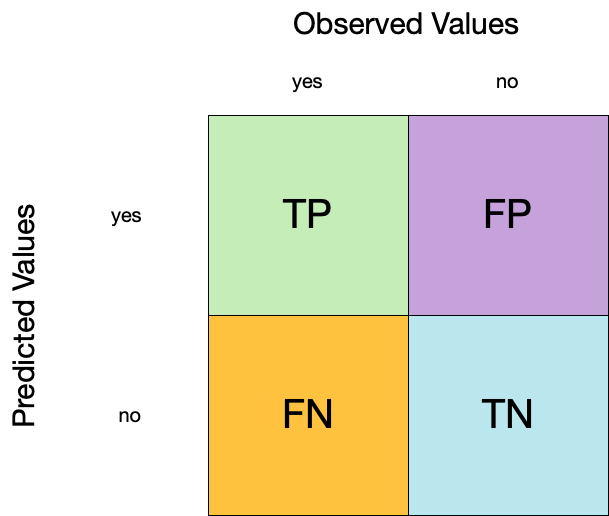
Confusion matrix ![]()
Confusion matrix ![]()

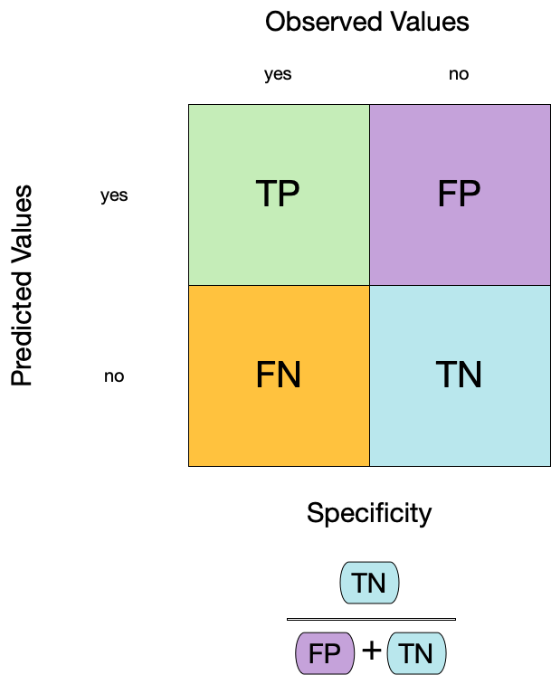
Metrics for model performance ![]()
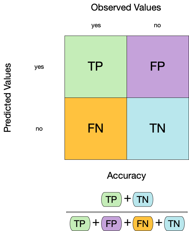
Metrics for model performance ![]()
Metrics for model performance ![]()
Metrics for model performance ![]()
We can use metric_set() to combine multiple calculations into one
forested_metrics <- metric_set(accuracy, specificity, sensitivity)
augment(forested_fit, new_data = forested_train) %>%
forested_metrics(truth = forested, estimate = .pred_class)
#> # A tibble: 3 × 3
#> .metric .estimator .estimate
#> <chr> <chr> <dbl>
#> 1 accuracy binary 0.944
#> 2 specificity binary 0.931
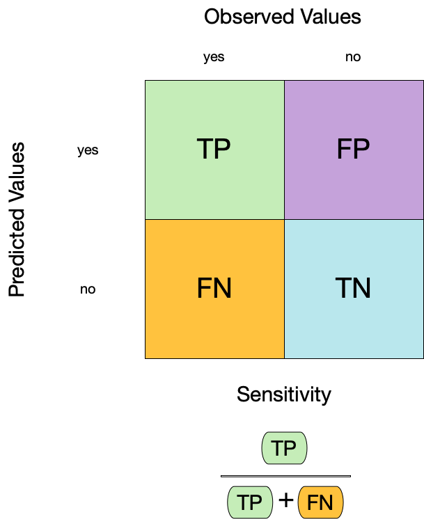
#> 3 sensitivity binary 0.954Metrics for model performance ![]()
Metrics and metric sets work with grouped data frames!
Your turn

Apply the forested_metrics metric set to augment()
output grouped by tree_no_tree.
Do any metrics differ substantially between groups?
05:00
Varying the threshold

ROC curves
For an ROC (receiver operator characteristic) curve, we plot
- the false positive rate (1 - specificity) on the x-axis
- the true positive rate (sensitivity) on the y-axis
with sensitivity and specificity calculated at all possible thresholds.

ROC curves
We can use the area under the ROC curve as a classification metric:
- ROC AUC = 1 💯
- ROC AUC = 1/2 😢

ROC curves ![]()
# Assumes _first_ factor level is event; there are options to change that
augment(forested_fit, new_data = forested_train) %>%
  roc_curve(truth = forested, .pred_Yes) %>%
  slice(1, 20, 50)
#> # A tibble: 3 × 3
#>   .threshold specificity sensitivity
#>        <dbl>       <dbl>       <dbl>
#> 1   -Inf           0           1
#> 2      0.235       0.885       0.972
#> 3      0.909       0.969       0.826

augment(forested_fit, new_data = forested_train) %>%
  roc_auc(truth = forested, .pred_Yes)
#> # A tibble: 1 × 3
#>   .metric .estimator .estimate
#>   <chr>   <chr>          <dbl>
#> 1 roc_auc binary         0.975
ROC curve plot ![]()

Your turn
Compute and plot an ROC curve for your current model.
What data are being used for this ROC curve plot?
05:00
Separation vs calibration
The ROC captures separation.

The Brier score captures calibration.

Dangers of overfitting

Dangers of overfitting ⚠️

Dangers of overfitting ⚠️ ![]()
forested_fit %>%
  augment(forested_train)
#> # A tibble: 5,685 × 22
#>    .pred_class .pred_Yes .pred_No forested  year elevation eastness northness
#>    <fct>           <dbl>    <dbl> <fct>    <dbl>     <dbl>    <dbl>     <dbl>
#>  1 No             0.0114   0.989  No        2016       464       -5       -99
#>  2 Yes            0.636    0.364  Yes       2016       166       92        37
#>  3 No             0.0114   0.989  No        2016       644      -85       -52
#>  4 Yes            0.977    0.0226 Yes       2014      1285        4        99
#>  5 Yes            0.977    0.0226 Yes       2013       822       87        48
#>  6 Yes            0.808    0.192  Yes       2017         3        6       -99
#>  7 Yes            0.977    0.0226 Yes       2014      2041      -95        28
#>  8 Yes            0.977    0.0226 Yes       2015      1009       -8        99
#>  9 No             0.0114   0.989  No        2017       436      -98        19
#> 10 No             0.0114   0.989  No        2018       775       63        76
#> # ℹ 5,675 more rows
#> # ℹ 14 more variables: roughness <dbl>, tree_no_tree <fct>, dew_temp <dbl>,
#> #   precip_annual <dbl>, temp_annual_mean <dbl>, temp_annual_min <dbl>,
#> #   temp_annual_max <dbl>, temp_january_min <dbl>, vapor_min <dbl>,
#> #   vapor_max <dbl>, canopy_cover <dbl>, lon <dbl>, lat <dbl>, land_type <fct>
We call this “resubstitution” or “repredicting the training set”
Dangers of overfitting ⚠️ ![]()
We call this a “resubstitution estimate”
Dangers of overfitting ⚠️ ![]()
Dangers of overfitting ⚠️ ![]()
⚠️ Remember that we’re demonstrating overfitting
⚠️ Don’t use the test set until the end of your modeling analysis
Your turn
Use augment() and a metric function to compute a classification metric like brier_class().
Compute the metrics for both training and testing data to demonstrate overfitting!
Notice the evidence of overfitting! ⚠️
05:00
Dangers of overfitting ⚠️ ![]()
What if we want to compare more models?
And/or more model configurations?
And we want to understand if these are important differences?
Cross-validation

Cross-validation

Your turn
If we use 10 folds, what percent of the training data
- ends up in analysis
- ends up in assessment
for each fold?

03:00
Cross-validation ![]()

vfold_cv(forested_train) # v = 10 is default
#> #  10-fold cross-validation
#> # A tibble: 10 × 2
#>    splits             id
#>    <list>             <chr>
#>  1 <split [5116/569]> Fold01
#>  2 <split [5116/569]> Fold02
#>  3 <split [5116/569]> Fold03
#>  4 <split [5116/569]> Fold04
#>  5 <split [5116/569]> Fold05
#>  6 <split [5117/568]> Fold06
#>  7 <split [5117/568]> Fold07
#>  8 <split [5117/568]> Fold08
#>  9 <split [5117/568]> Fold09
#> 10 <split [5117/568]> Fold10
Cross-validation ![]()
What is in this?
Cross-validation ![]()
Cross-validation ![]()
We’ll use this setup:
set.seed(123)
forested_folds <- vfold_cv(forested_train, v = 10)
forested_folds
#> #  10-fold cross-validation
#> # A tibble: 10 × 2
#>    splits             id
#>    <list>             <chr>
#>  1 <split [5116/569]> Fold01
#>  2 <split [5116/569]> Fold02
#>  3 <split [5116/569]> Fold03
#>  4 <split [5116/569]> Fold04
#>  5 <split [5116/569]> Fold05
#>  6 <split [5117/568]> Fold06
#>  7 <split [5117/568]> Fold07
#>  8 <split [5117/568]> Fold08
#>  9 <split [5117/568]> Fold09
#> 10 <split [5117/568]> Fold10
Set the seed when creating resamples
Evaluating model performance ![]()

forested_res %>%
  collect_metrics()
#> # A tibble: 3 × 6
#>   .metric     .estimator   mean     n std_err .config
#>   <chr>       <chr>       <dbl> <int>   <dbl> <chr>
#> 1 accuracy    binary     0.894     10 0.00562 Preprocessor1_Model1
#> 2 brier_class binary     0.0817    10 0.00434 Preprocessor1_Model1
#> 3 roc_auc binary 0.951 10 0.00378 Preprocessor1_Model1We can reliably measure performance using only the training data 🎉
Comparing metrics ![]()
How do the metrics from resampling compare to the metrics from training and testing?
The ROC AUC previously was
- 0.97 for the training set
- 0.95 for test set
Remember that:
⚠️ the training set gives you overly optimistic metrics
⚠️ the test set is precious
Evaluating model performance ![]()
# Save the assessment set results
ctrl_forested <- control_resamples(save_pred = TRUE)
forested_res <- fit_resamples(forested_wflow, forested_folds, control = ctrl_forested)

forested_res
#> # Resampling results
#> # 10-fold cross-validation
#> # A tibble: 10 × 5
#>    splits             id     .metrics         .notes           .predictions
#>    <list>             <chr>  <list>           <list>           <list>
#>  1 <split [5116/569]> Fold01 <tibble [3 × 4]> <tibble [0 × 3]> <tibble>
#>  2 <split [5116/569]> Fold02 <tibble [3 × 4]> <tibble [0 × 3]> <tibble>
#>  3 <split [5116/569]> Fold03 <tibble [3 × 4]> <tibble [0 × 3]> <tibble>
#>  4 <split [5116/569]> Fold04 <tibble [3 × 4]> <tibble [0 × 3]> <tibble>
#>  5 <split [5116/569]> Fold05 <tibble [3 × 4]> <tibble [0 × 3]> <tibble>
#>  6 <split [5117/568]> Fold06 <tibble [3 × 4]> <tibble [0 × 3]> <tibble>
#>  7 <split [5117/568]> Fold07 <tibble [3 × 4]> <tibble [0 × 3]> <tibble>
#>  8 <split [5117/568]> Fold08 <tibble [3 × 4]> <tibble [0 × 3]> <tibble>
#>  9 <split [5117/568]> Fold09 <tibble [3 × 4]> <tibble [0 × 3]> <tibble>
#> 10 <split [5117/568]> Fold10 <tibble [3 × 4]> <tibble [0 × 3]> <tibble>
Evaluating model performance ![]()
# Save the assessment set results
forested_preds <- collect_predictions(forested_res)
forested_preds
#> # A tibble: 5,685 × 7
#>    .pred_class .pred_Yes .pred_No id      .row forested .config
#>    <fct>           <dbl>    <dbl> <chr>  <int> <fct>    <chr>
#>  1 Yes           0.5       0.5    Fold01     2 Yes      Preprocessor1_Model1
#>  2 Yes           0.982     0.0178 Fold01     5 Yes      Preprocessor1_Model1
#>  3 No            0.00790   0.992  Fold01     9 No       Preprocessor1_Model1
#>  4 No            0.4       0.6    Fold01    14 No       Preprocessor1_Model1
#>  5 Yes           0.870     0.130  Fold01    18 Yes      Preprocessor1_Model1
#>  6 Yes           0.982     0.0178 Fold01    59 Yes      Preprocessor1_Model1
#>  7 No            0.00790   0.992  Fold01    67 No       Preprocessor1_Model1
#>  8 Yes           0.982     0.0178 Fold01    89 Yes      Preprocessor1_Model1
#>  9 No            0.00790   0.992  Fold01    94 No       Preprocessor1_Model1
#> 10 Yes           0.982     0.0178 Fold01   111 Yes      Preprocessor1_Model1
#> # ℹ 5,675 more rows
Evaluating model performance ![]()
forested_preds %>%
  group_by(id) %>%
  forested_metrics(truth = forested, estimate = .pred_class)
#> # A tibble: 30 × 4
#>    id     .metric  .estimator .estimate
#>    <chr>  <chr>    <chr>          <dbl>
#>  1 Fold01 accuracy binary         0.896
#>  2 Fold02 accuracy binary         0.859
#>  3 Fold03 accuracy binary         0.868
#>  4 Fold04 accuracy binary         0.921
#>  5 Fold05 accuracy binary         0.900
#>  6 Fold06 accuracy binary         0.891
#>  7 Fold07 accuracy binary         0.896
#>  8 Fold08 accuracy binary         0.903
#>  9 Fold09 accuracy binary         0.896
#> 10 Fold10 accuracy binary         0.905
#> # ℹ 20 more rows
Where are the fitted models? ![]()
forested_res
#> # Resampling results
#> # 10-fold cross-validation
#> # A tibble: 10 × 5
#>    splits             id     .metrics         .notes           .predictions
#>    <list>             <chr>  <list>           <list>           <list>
#>  1 <split [5116/569]> Fold01 <tibble [3 × 4]> <tibble [0 × 3]> <tibble>
#>  2 <split [5116/569]> Fold02 <tibble [3 × 4]> <tibble [0 × 3]> <tibble>
#>  3 <split [5116/569]> Fold03 <tibble [3 × 4]> <tibble [0 × 3]> <tibble>
#>  4 <split [5116/569]> Fold04 <tibble [3 × 4]> <tibble [0 × 3]> <tibble>
#>  5 <split [5116/569]> Fold05 <tibble [3 × 4]> <tibble [0 × 3]> <tibble>
#>  6 <split [5117/568]> Fold06 <tibble [3 × 4]> <tibble [0 × 3]> <tibble>
#>  7 <split [5117/568]> Fold07 <tibble [3 × 4]> <tibble [0 × 3]> <tibble>
#>  8 <split [5117/568]> Fold08 <tibble [3 × 4]> <tibble [0 × 3]> <tibble>
#>  9 <split [5117/568]> Fold09 <tibble [3 × 4]> <tibble [0 × 3]> <tibble>
#> 10 <split [5117/568]> Fold10 <tibble [3 × 4]> <tibble [0 × 3]> <tibble>
🗑️
Bootstrapping

Bootstrapping ![]()
set.seed(3214)
bootstraps(forested_train)
#> # Bootstrap sampling
#> # A tibble: 25 × 2
#>    splits              id
#>    <list>              <chr>
#>  1 <split [5685/2075]> Bootstrap01
#>  2 <split [5685/2093]> Bootstrap02
#>  3 <split [5685/2129]> Bootstrap03
#>  4 <split [5685/2093]> Bootstrap04
#>  5 <split [5685/2111]> Bootstrap05
#>  6 <split [5685/2105]> Bootstrap06
#>  7 <split [5685/2139]> Bootstrap07
#>  8 <split [5685/2079]> Bootstrap08
#>  9 <split [5685/2113]> Bootstrap09
#> 10 <split [5685/2101]> Bootstrap10
#> # ℹ 15 more rows
The whole game - status update
Your turn
Create:
- Monte Carlo Cross-Validation sets
- validation set
(use the reference guide to find the functions)
Don’t forget to set a seed when you resample!
05:00
Monte Carlo Cross-Validation ![]()
set.seed(322)
mc_cv(forested_train, times = 10)
#> # Monte Carlo cross-validation (0.75/0.25) with 10 resamples
#> # A tibble: 10 × 2
#>    splits              id
#>    <list>              <chr>
#>  1 <split [4263/1422]> Resample01
#>  2 <split [4263/1422]> Resample02
#>  3 <split [4263/1422]> Resample03
#>  4 <split [4263/1422]> Resample04
#>  5 <split [4263/1422]> Resample05
#>  6 <split [4263/1422]> Resample06
#>  7 <split [4263/1422]> Resample07
#>  8 <split [4263/1422]> Resample08
#>  9 <split [4263/1422]> Resample09
#> 10 <split [4263/1422]> Resample10
Validation set ![]()
A validation set is just another type of resample
Create a random forest model ![]()

Create a random forest model ![]()

rf_wflow <- workflow(forested ~ ., rf_spec)
rf_wflow
#> ══ Workflow ══════════════════════════════════════════════════════════
#> Preprocessor: Formula
#> Model: rand_forest()
#>
#> ── Preprocessor ──────────────────────────────────────────────────────
#> forested ~ .
#>
#> ── Model ─────────────────────────────────────────────────────────────
#> Random Forest Model Specification (classification)
#>
#> Main Arguments:
#>   trees = 1000
#>
#> Computational engine: ranger
Your turn
Use fit_resamples() and rf_wflow to:
- keep predictions
- compute metrics
08:00
Evaluating model performance ![]()
ctrl_forested <- control_resamples(save_pred = TRUE)

# Random forest uses random numbers so set the seed first

set.seed(2)
rf_res <- fit_resamples(rf_wflow, forested_folds, control = ctrl_forested)
collect_metrics(rf_res)
#> # A tibble: 3 × 6
#>   .metric     .estimator   mean     n std_err .config
#>   <chr>       <chr>       <dbl> <int>   <dbl> <chr>
#> 1 accuracy    binary     0.918     10 0.00585 Preprocessor1_Model1
#> 2 brier_class binary     0.0618    10 0.00337 Preprocessor1_Model1
#> 3 roc_auc     binary     0.972     10 0.00309 Preprocessor1_Model1
The whole game - status update
The final fit ![]()
Suppose that we are happy with our random forest model.
Let’s fit the model on the training set and verify our performance using the test set.
We’ve shown you fit() and predict() (+ augment()) but there is a shortcut:
# forested_split has train + test info
final_fit <- last_fit(rf_wflow, forested_split)

final_fit
#> # Resampling results
#> # Manual resampling
#> # A tibble: 1 × 6
#>   splits              id               .metrics .notes   .predictions .workflow
#>   <list>              <chr>            <list>   <list>   <list>       <list>
#> 1 <split [5685/1422]> train/test split <tibble> <tibble> <tibble>     <workflow>
What is in final_fit? ![]()
These are metrics computed with the test set
What is in final_fit? ![]()
collect_predictions(final_fit)
#> # A tibble: 1,422 × 7
#>    .pred_class .pred_Yes .pred_No id                .row forested .config
#>    <fct>           <dbl>    <dbl> <chr>            <int> <fct>    <chr>
#>  1 Yes             0.822   0.178  train/test split     3 No       Preprocessor1…
#>  2 Yes             0.707   0.293  train/test split     4 Yes      Preprocessor1…
#>  3 No              0.270   0.730  train/test split     7 Yes      Preprocessor1…
#>  4 Yes             0.568   0.432  train/test split     8 Yes      Preprocessor1…
#>  5 Yes             0.554   0.446  train/test split    10 Yes      Preprocessor1…
#>  6 Yes             0.970   0.0297 train/test split    11 Yes      Preprocessor1…
#>  7 Yes             0.963   0.0367 train/test split    12 Yes      Preprocessor1…
#>  8 Yes             0.947   0.0528 train/test split    14 Yes      Preprocessor1…
#>  9 Yes             0.943   0.0573 train/test split    15 Yes      Preprocessor1…
#> 10 Yes             0.977   0.0227 train/test split    19 Yes      Preprocessor1…
#> # ℹ 1,412 more rows
What is in final_fit? ![]()
extract_workflow(final_fit)
#> ══ Workflow [trained] ════════════════════════════════════════════════
#> Preprocessor: Formula
#> Model: rand_forest()
#>
#> ── Preprocessor ──────────────────────────────────────────────────────
#> forested ~ .
#>
#> ── Model ─────────────────────────────────────────────────────────────
#> Ranger result
#>
#> Call:
#>  ranger::ranger(x = maybe_data_frame(x), y = y, num.trees = ~1000,      num.threads = 1, verbose = FALSE, seed = sample.int(10^5,          1), probability = TRUE)
#>
#> Type:                             Probability estimation
#> Number of trees:                  1000
#> Sample size:                      5685
#> Number of independent variables:  18
#> Mtry:                             4
#> Target node size:                 10
#> Variable importance mode:         none
#> Splitrule:                        gini
#> OOB prediction error (Brier s.):  0.06153207
Use this for prediction on new data, like for deploying
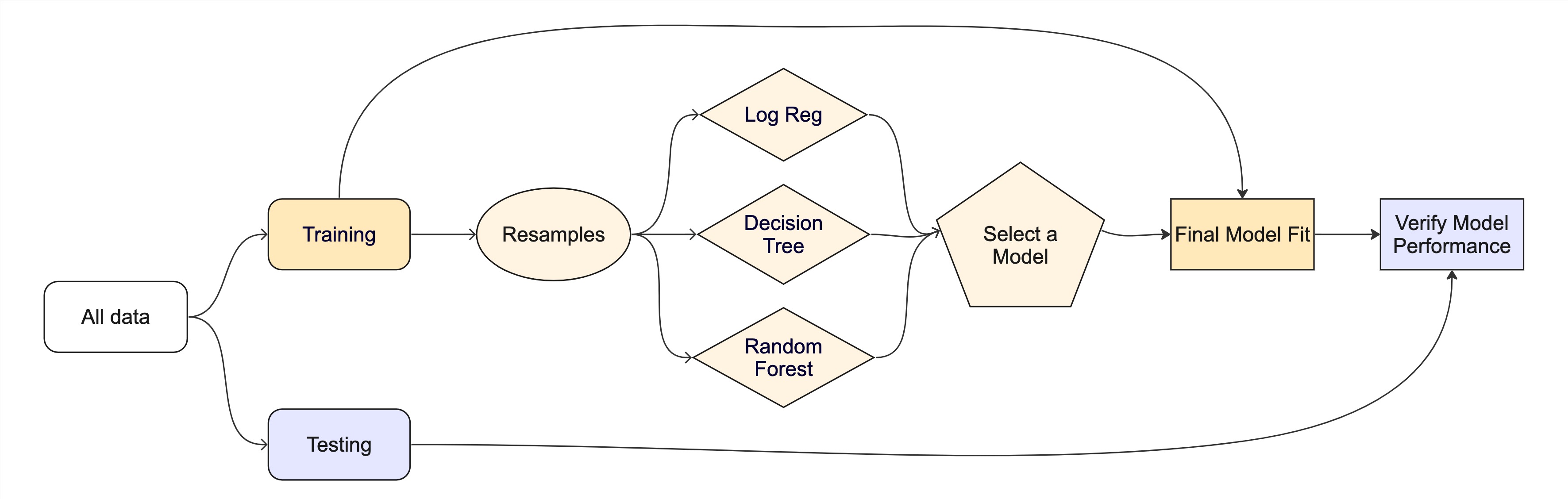
The whole game