augment(taxi_fit, new_data = taxi_train) %>%
  relocate(tip, .pred_class, .pred_yes, .pred_no)
#> # A tibble: 8,000 × 10
#>    tip   .pred_class .pred_yes .pred_no distance company local dow   month  hour
#>    <fct> <fct>           <dbl>    <dbl>    <dbl> <fct>   <fct> <fct> <fct> <int>
#>  1 yes   yes             0.967   0.0333    17.2  Chicag… no    Thu   Feb      16
#>  2 yes   yes             0.935   0.0646     0.88 City S… yes   Thu   Mar       8
#>  3 yes   yes             0.967   0.0333    18.1  other   no    Mon   Feb      18
#>  4 yes   yes             0.949   0.0507    12.2  Chicag… no    Sun   Mar      21
#>  5 yes   yes             0.821   0.179      0.94 Sun Ta… yes   Sat   Apr      23
#>  6 yes   yes             0.967   0.0333    17.5  Flash … no    Fri   Mar      12
#>  7 yes   yes             0.967   0.0333    17.7  other   no    Sun   Jan       6
#>  8 yes   yes             0.938   0.0616     1.85 Taxica… no    Fri   Apr      12
#>  9 yes   yes             0.938   0.0616     0.53 Sun Ta… no    Tue   Mar      18
#> 10 yes   yes             0.931   0.0694     6.65 Taxica… no    Sun   Apr      11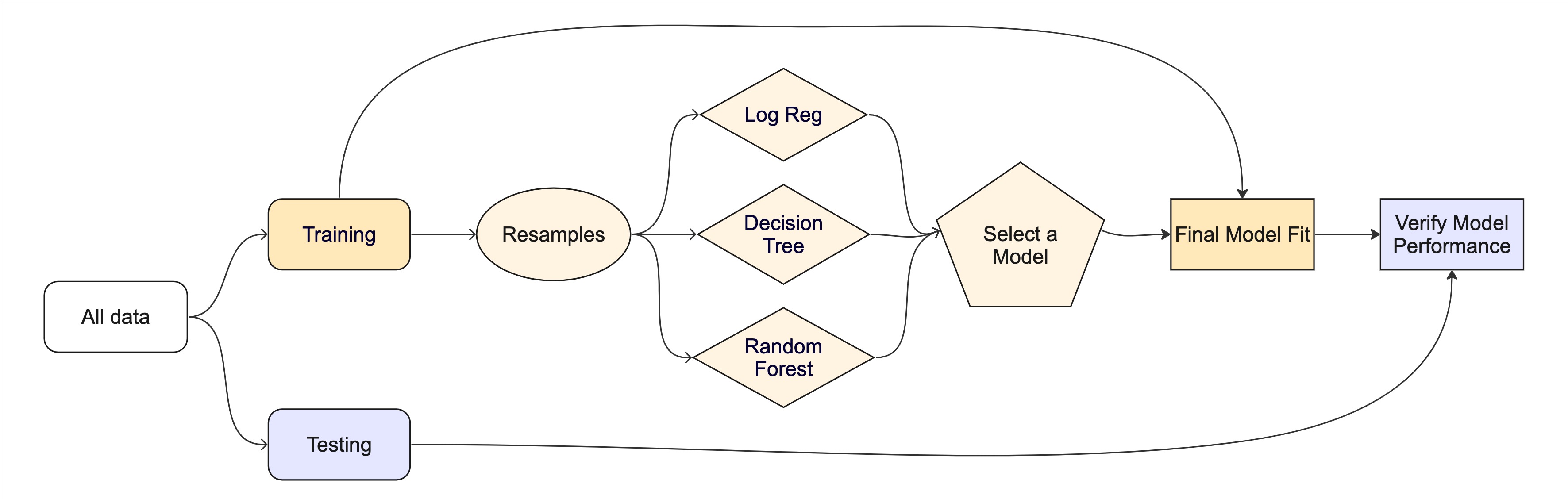
#> # ℹ 7,990 more rows4 - Evaluating models
Introduction to tidymodels
Confusion matrix ![]()

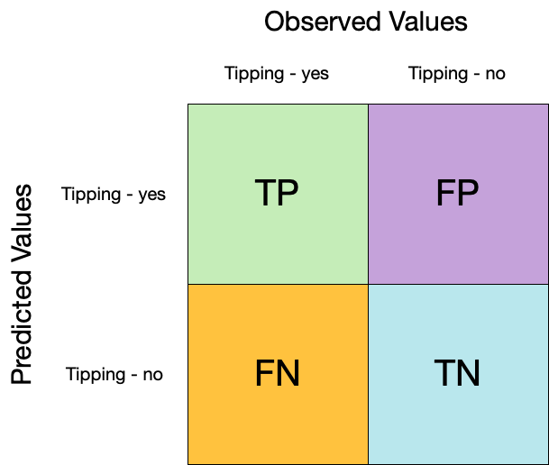
Confusion matrix ![]()
Confusion matrix ![]()

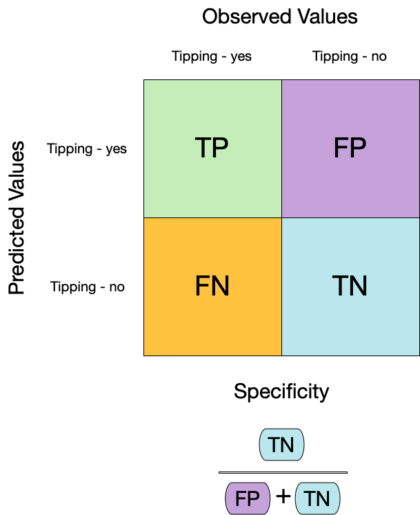
Metrics for model performance ![]()
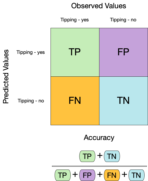
Dangers of accuracy ![]()
We need to be careful of using accuracy() since it can give “good” performance by only predicting one way with imbalanced data
Metrics for model performance ![]()
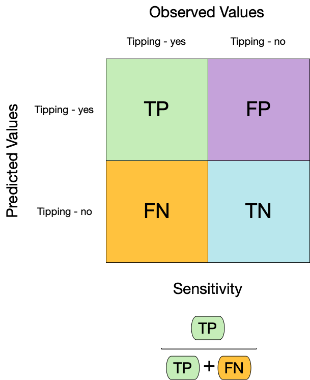
Metrics for model performance ![]()
Metrics for model performance ![]()
We can use metric_set() to combine multiple calculations into one
taxi_metrics <- metric_set(accuracy, specificity, sensitivity)

augment(taxi_fit, new_data = taxi_train) %>%
  taxi_metrics(truth = tip, estimate = .pred_class)
#> # A tibble: 3 × 3
#>   .metric     .estimator .estimate
#>   <chr>       <chr>          <dbl>
#> 1 accuracy    binary         0.928
#> 2 specificity binary         0.130
#> 3 sensitivity binary         0.994
Metrics for model performance ![]()
taxi_metrics <- metric_set(accuracy, specificity, sensitivity)

augment(taxi_fit, new_data = taxi_train) %>%
  group_by(local) %>%
  taxi_metrics(truth = tip, estimate = .pred_class)
#> # A tibble: 6 × 4
#>   local .metric     .estimator .estimate
#>   <fct> <chr>       <chr>          <dbl>
#> 1 yes   accuracy    binary         0.898
#> 2 no    accuracy    binary         0.935
#> 3 yes   specificity binary         0.169
#> 4 no    specificity binary         0.116
#> 5 yes   sensitivity binary         0.987
#> 6 no sensitivity binary 0.996Varying the threshold

ROC curves ![]()
# Assumes _first_ factor level is event; there are options to change that
augment(taxi_fit, new_data = taxi_train) %>%
  roc_curve(truth = tip, .pred_yes) %>%
  slice(1, 20, 50)
#> # A tibble: 3 × 3
#>   .threshold specificity sensitivity
#>        <dbl>       <dbl>       <dbl>
#> 1   -Inf           0         1
#> 2      0.783       0.209     0.981
#> 3      1           1         0.00135

augment(taxi_fit, new_data = taxi_train) %>%
  roc_auc(truth = tip, .pred_yes)
#> # A tibble: 1 × 3
#>   .metric .estimator .estimate
#>   <chr>   <chr>          <dbl>
#> 1 roc_auc binary         0.691
ROC curve plot ![]()

Your turn

Compute and plot an ROC curve for your current model.
What data are being used for this ROC curve plot?
05:00
Dangers of overfitting ⚠️

Dangers of overfitting ⚠️

Dangers of overfitting ⚠️ ![]()
taxi_fit %>%
  augment(taxi_train)
#> # A tibble: 8,000 × 10
#>    tip   distance company local dow   month  hour .pred_class .pred_yes .pred_no
#>    <fct>    <dbl> <fct>   <fct> <fct> <fct> <int> <fct>           <dbl>    <dbl>
#>  1 yes      17.2  Chicag… no    Thu   Feb      16 yes             0.967   0.0333
#>  2 yes       0.88 City S… yes   Thu   Mar       8 yes             0.935   0.0646
#>  3 yes      18.1  other   no    Mon   Feb      18 yes             0.967   0.0333
#>  4 yes      12.2  Chicag… no    Sun   Mar      21 yes             0.949   0.0507
#>  5 yes       0.94 Sun Ta… yes   Sat   Apr      23 yes             0.821   0.179
#>  6 yes      17.5  Flash … no    Fri   Mar      12 yes             0.967   0.0333
#>  7 yes      17.7  other   no    Sun   Jan       6 yes             0.967   0.0333
#>  8 yes       1.85 Taxica… no    Fri   Apr      12 yes             0.938   0.0616
#>  9 yes       0.53 Sun Ta… no    Tue   Mar      18 yes             0.938   0.0616
#> 10 yes       6.65 Taxica… no    Sun   Apr      11 yes             0.931   0.0694
#> # ℹ 7,990 more rows
We call this “resubstitution” or “repredicting the training set”
Dangers of overfitting ⚠️ ![]()
We call this a “resubstitution estimate”
Dangers of overfitting ⚠️ ![]()
Dangers of overfitting ⚠️ ![]()
⚠️ Remember that we’re demonstrating overfitting
⚠️ Don’t use the test set until the end of your modeling analysis
Your turn
Use augment() and a metric function to compute a classification metric like brier_class().
Compute the metrics for both training and testing data to demonstrate overfitting!
Notice the evidence of overfitting! ⚠️
05:00
Dangers of overfitting ⚠️ ![]()
What if we want to compare more models?
And/or more model configurations?
And we want to understand if these are important differences?
Cross-validation

Cross-validation

Your turn
If we use 10 folds, what percent of the training data
- ends up in analysis
- ends up in assessment
for each fold?

03:00
Cross-validation ![]()

vfold_cv(taxi_train) # v = 10 is default
#> #  10-fold cross-validation
#> # A tibble: 10 × 2
#>    splits             id
#>    <list>             <chr>
#>  1 <split [7200/800]> Fold01
#>  2 <split [7200/800]> Fold02
#>  3 <split [7200/800]> Fold03
#>  4 <split [7200/800]> Fold04
#>  5 <split [7200/800]> Fold05
#>  6 <split [7200/800]> Fold06
#>  7 <split [7200/800]> Fold07
#>  8 <split [7200/800]> Fold08
#>  9 <split [7200/800]> Fold09
#> 10 <split [7200/800]> Fold10
Cross-validation ![]()
What is in this?
Cross-validation ![]()
Cross-validation ![]()
vfold_cv(taxi_train, strata = tip)
#> #  10-fold cross-validation using stratification
#> # A tibble: 10 × 2
#>    splits             id
#>    <list>             <chr>
#>  1 <split [7200/800]> Fold01
#>  2 <split [7200/800]> Fold02
#>  3 <split [7200/800]> Fold03
#>  4 <split [7200/800]> Fold04
#>  5 <split [7200/800]> Fold05
#>  6 <split [7200/800]> Fold06
#>  7 <split [7200/800]> Fold07
#>  8 <split [7200/800]> Fold08
#>  9 <split [7200/800]> Fold09
#> 10 <split [7200/800]> Fold10
Stratification often helps, with very little downside
Cross-validation ![]()
We’ll use this setup:
set.seed(123)
taxi_folds <- vfold_cv(taxi_train, v = 10, strata = tip)
taxi_folds
#> #  10-fold cross-validation using stratification
#> # A tibble: 10 × 2
#>    splits             id
#>    <list>             <chr>
#>  1 <split [7200/800]> Fold01
#>  2 <split [7200/800]> Fold02
#>  3 <split [7200/800]> Fold03
#>  4 <split [7200/800]> Fold04
#>  5 <split [7200/800]> Fold05
#>  6 <split [7200/800]> Fold06
#>  7 <split [7200/800]> Fold07
#>  8 <split [7200/800]> Fold08
#>  9 <split [7200/800]> Fold09
#> 10 <split [7200/800]> Fold10
Set the seed when creating resamples
Evaluating model performance ![]()

We can reliably measure performance using only the training data 🎉
Comparing metrics ![]()
How do the metrics from resampling compare to the metrics from training and testing?
The ROC AUC previously was
- 0.69 for the training set
- 0.64 for test set
Remember that:
⚠️ the training set gives you overly optimistic metrics
⚠️ the test set is precious
Evaluating model performance ![]()
# Save the assessment set results
ctrl_taxi <- control_resamples(save_pred = TRUE)
taxi_res <- fit_resamples(taxi_wflow, taxi_folds, control = ctrl_taxi)

taxi_res
#> # Resampling results
#> # 10-fold cross-validation using stratification
#> # A tibble: 10 × 5
#>    splits             id     .metrics         .notes           .predictions
#>    <list>             <chr>  <list>           <list>           <list>
#>  1 <split [7200/800]> Fold01 <tibble [2 × 4]> <tibble [0 × 3]> <tibble>
#>  2 <split [7200/800]> Fold02 <tibble [2 × 4]> <tibble [0 × 3]> <tibble>
#>  3 <split [7200/800]> Fold03 <tibble [2 × 4]> <tibble [0 × 3]> <tibble>
#>  4 <split [7200/800]> Fold04 <tibble [2 × 4]> <tibble [0 × 3]> <tibble>
#>  5 <split [7200/800]> Fold05 <tibble [2 × 4]> <tibble [0 × 3]> <tibble>
#>  6 <split [7200/800]> Fold06 <tibble [2 × 4]> <tibble [0 × 3]> <tibble>
#>  7 <split [7200/800]> Fold07 <tibble [2 × 4]> <tibble [0 × 3]> <tibble>
#>  8 <split [7200/800]> Fold08 <tibble [2 × 4]> <tibble [0 × 3]> <tibble>
#>  9 <split [7200/800]> Fold09 <tibble [2 × 4]> <tibble [0 × 3]> <tibble>
#> 10 <split [7200/800]> Fold10 <tibble [2 × 4]> <tibble [0 × 3]> <tibble>
Evaluating model performance ![]()
# Save the assessment set results
taxi_preds <- collect_predictions(taxi_res)
taxi_preds
#> # A tibble: 8,000 × 7
#>    id     .pred_yes .pred_no  .row .pred_class tip   .config
#>    <chr>      <dbl>    <dbl> <int> <fct>       <fct> <chr>
#>  1 Fold01     0.938   0.0615    14 yes         yes   Preprocessor1_Model1
#>  2 Fold01     0.946   0.0544    19 yes         yes   Preprocessor1_Model1
#>  3 Fold01     0.973   0.0269    33 yes         yes   Preprocessor1_Model1
#>  4 Fold01     0.903   0.0971    43 yes         yes   Preprocessor1_Model1
#>  5 Fold01     0.973   0.0269    74 yes         yes   Preprocessor1_Model1
#>  6 Fold01     0.903   0.0971   103 yes         yes   Preprocessor1_Model1
#>  7 Fold01     0.915   0.0851   104 yes         no    Preprocessor1_Model1
#>  8 Fold01     0.903   0.0971   124 yes         yes   Preprocessor1_Model1
#>  9 Fold01     0.667   0.333    126 yes         yes   Preprocessor1_Model1
#> 10 Fold01     0.949   0.0510   128 yes         yes   Preprocessor1_Model1
#> # ℹ 7,990 more rows
Evaluating model performance ![]()
taxi_preds %>%
  group_by(id) %>%
  taxi_metrics(truth = tip, estimate = .pred_class)
#> # A tibble: 30 × 4
#>    id     .metric  .estimator .estimate
#>    <chr>  <chr>    <chr>          <dbl>
#>  1 Fold01 accuracy binary         0.905
#>  2 Fold02 accuracy binary         0.925
#>  3 Fold03 accuracy binary         0.926
#>  4 Fold04 accuracy binary         0.915
#>  5 Fold05 accuracy binary         0.902
#>  6 Fold06 accuracy binary         0.912
#>  7 Fold07 accuracy binary         0.906
#>  8 Fold08 accuracy binary         0.91
#>  9 Fold09 accuracy binary         0.918
#> 10 Fold10 accuracy binary         0.931
#> # ℹ 20 more rows
Where are the fitted models? ![]()
taxi_res
#> # Resampling results
#> # 10-fold cross-validation using stratification
#> # A tibble: 10 × 5
#>    splits             id     .metrics         .notes           .predictions
#>    <list>             <chr>  <list>           <list>           <list>
#>  1 <split [7200/800]> Fold01 <tibble [2 × 4]> <tibble [0 × 3]> <tibble>
#>  2 <split [7200/800]> Fold02 <tibble [2 × 4]> <tibble [0 × 3]> <tibble>
#>  3 <split [7200/800]> Fold03 <tibble [2 × 4]> <tibble [0 × 3]> <tibble>
#>  4 <split [7200/800]> Fold04 <tibble [2 × 4]> <tibble [0 × 3]> <tibble>
#>  5 <split [7200/800]> Fold05 <tibble [2 × 4]> <tibble [0 × 3]> <tibble>
#>  6 <split [7200/800]> Fold06 <tibble [2 × 4]> <tibble [0 × 3]> <tibble>
#>  7 <split [7200/800]> Fold07 <tibble [2 × 4]> <tibble [0 × 3]> <tibble>
#>  8 <split [7200/800]> Fold08 <tibble [2 × 4]> <tibble [0 × 3]> <tibble>
#>  9 <split [7200/800]> Fold09 <tibble [2 × 4]> <tibble [0 × 3]> <tibble>
#> 10 <split [7200/800]> Fold10 <tibble [2 × 4]> <tibble [0 × 3]> <tibble>
🗑️
Bootstrapping

Bootstrapping ![]()
set.seed(3214)
bootstraps(taxi_train)
#> # Bootstrap sampling
#> # A tibble: 25 × 2
#>    splits              id
#>    <list>              <chr>
#>  1 <split [8000/2902]> Bootstrap01
#>  2 <split [8000/2916]> Bootstrap02
#>  3 <split [8000/3004]> Bootstrap03
#>  4 <split [8000/2979]> Bootstrap04
#>  5 <split [8000/2961]> Bootstrap05
#>  6 <split [8000/2962]> Bootstrap06
#>  7 <split [8000/3026]> Bootstrap07
#>  8 <split [8000/2926]> Bootstrap08
#>  9 <split [8000/2972]> Bootstrap09
#> 10 <split [8000/2972]> Bootstrap10
#> # ℹ 15 more rows
The whole game - status update
Your turn
Create:
- Monte Carlo Cross-Validation sets
- validation set
(use the reference guide to find the functions)
Don’t forget to set a seed when you resample!
05:00
Monte Carlo Cross-Validation ![]()
set.seed(322)
mc_cv(taxi_train, times = 10)
#> # Monte Carlo cross-validation (0.75/0.25) with 10 resamples
#> # A tibble: 10 × 2
#>    splits              id
#>    <list>              <chr>
#>  1 <split [6000/2000]> Resample01
#>  2 <split [6000/2000]> Resample02
#>  3 <split [6000/2000]> Resample03
#>  4 <split [6000/2000]> Resample04
#>  5 <split [6000/2000]> Resample05
#>  6 <split [6000/2000]> Resample06
#>  7 <split [6000/2000]> Resample07
#>  8 <split [6000/2000]> Resample08
#>  9 <split [6000/2000]> Resample09
#> 10 <split [6000/2000]> Resample10
Validation set ![]()
A validation set is just another type of resample
Create a random forest model ![]()

Create a random forest model ![]()

rf_wflow <- workflow(tip ~ ., rf_spec)
rf_wflow
#> ══ Workflow ══════════════════════════════════════════════════════════
#> Preprocessor: Formula
#> Model: rand_forest()
#>
#> ── Preprocessor ──────────────────────────────────────────────────────
#> tip ~ .
#>
#> ── Model ─────────────────────────────────────────────────────────────
#> Random Forest Model Specification (classification)
#>
#> Main Arguments:
#>   trees = 1000
#>
#> Computational engine: ranger
Your turn
Use fit_resamples() and rf_wflow to:
- keep predictions
- compute metrics
08:00
Evaluating model performance ![]()
ctrl_taxi <- control_resamples(save_pred = TRUE)

# Random forest uses random numbers so set the seed first

set.seed(2)
rf_res <- fit_resamples(rf_wflow, taxi_folds, control = ctrl_taxi)
collect_metrics(rf_res)
#> # A tibble: 2 × 6
#>   .metric  .estimator  mean     n std_err .config
#>   <chr>    <chr>      <dbl> <int>   <dbl> <chr>
#> 1 accuracy binary     0.923    10 0.00317 Preprocessor1_Model1
#> 2 roc_auc  binary     0.616    10 0.0147  Preprocessor1_Model1
The whole game - status update
The final fit ![]()
Suppose that we are happy with our random forest model.
Let’s fit the model on the training set and verify our performance using the test set.
We’ve shown you fit() and predict() (+ augment()) but there is a shortcut:
# taxi_split has train + test info
final_fit <- last_fit(rf_wflow, taxi_split)

final_fit
#> # Resampling results
#> # Manual resampling
#> # A tibble: 1 × 6
#>   splits              id               .metrics .notes   .predictions .workflow
#>   <list>              <chr>            <list>   <list>   <list>       <list>
#> 1 <split [8000/2000]> train/test split <tibble> <tibble> <tibble>     <workflow>
What is in final_fit? ![]()
These are metrics computed with the test set
What is in final_fit? ![]()
collect_predictions(final_fit)
#> # A tibble: 2,000 × 7
#>    id               .pred_yes .pred_no  .row .pred_class tip   .config
#>    <chr>                <dbl>    <dbl> <int> <fct>       <fct> <chr>
#>  1 train/test split     0.957   0.0426     4 yes         yes   Preprocessor1_Mo…
#>  2 train/test split     0.938   0.0621    10 yes         yes   Preprocessor1_Mo…
#>  3 train/test split     0.958   0.0416    19 yes         yes   Preprocessor1_Mo…
#>  4 train/test split     0.894   0.106     23 yes         yes   Preprocessor1_Mo…
#>  5 train/test split     0.943   0.0573    28 yes         yes   Preprocessor1_Mo…
#>  6 train/test split     0.979   0.0213    34 yes         yes   Preprocessor1_Mo…
#>  7 train/test split     0.954   0.0463    35 yes         yes   Preprocessor1_Mo…
#>  8 train/test split     0.928   0.0722    38 yes         yes   Preprocessor1_Mo…
#>  9 train/test split     0.985   0.0147    40 yes         yes   Preprocessor1_Mo…
#> 10 train/test split     0.948   0.0523    42 yes         no    Preprocessor1_Mo…
#> # ℹ 1,990 more rows
What is in final_fit? ![]()
extract_workflow(final_fit)
#> ══ Workflow [trained] ════════════════════════════════════════════════
#> Preprocessor: Formula
#> Model: rand_forest()
#>
#> ── Preprocessor ──────────────────────────────────────────────────────
#> tip ~ .
#>
#> ── Model ─────────────────────────────────────────────────────────────
#> Ranger result
#>
#> Call:
#>  ranger::ranger(x = maybe_data_frame(x), y = y, num.trees = ~1000,      num.threads = 1, verbose = FALSE, seed = sample.int(10^5,          1), probability = TRUE)
#>
#> Type:                             Probability estimation
#> Number of trees:                  1000
#> Sample size:                      8000
#> Number of independent variables:  6
#> Mtry:                             2
#> Target node size:                 10
#> Variable importance mode:         none
#> Splitrule:                        gini
#> OOB prediction error (Brier s.):  0.07069778
Use this for prediction on new data, like for deploying
The whole game