2 - Tuning Hyperparameters

Advanced tidymodels

Previously - Setup

library(tidymodels)
library(textrecipes)
library(bonsai)

# Max's usual settings: 
tidymodels_prefer()
theme_set(theme_bw())
options(
  pillar.advice = FALSE, 
  pillar.min_title_chars = Inf
)

reg_metrics <- metric_set(mae, rsq)

data(hotel_rates)
set.seed(295)
hotel_rates <- 
  hotel_rates %>% 
  sample_n(5000) %>% 
  arrange(arrival_date) %>% 
  select(-arrival_date) %>% 
  mutate(
    company = factor(as.character(company)),
    country = factor(as.character(country)),
    agent = factor(as.character(agent))
  )

Previously - Data Usage

set.seed(4028)
hotel_split <- initial_split(hotel_rates, strata = avg_price_per_room)

hotel_train <- training(hotel_split)
hotel_test <- testing(hotel_split)

set.seed(472)
hotel_rs <- vfold_cv(hotel_train, strata = avg_price_per_room)

Previously - Feature engineering

library(textrecipes)

hash_rec <-
  recipe(avg_price_per_room ~ ., data = hotel_train) %>%
  step_YeoJohnson(lead_time) %>%
  # Defaults to 32 signed indicator columns
  step_dummy_hash(agent) %>%
  step_dummy_hash(company) %>%
  # Regular indicators for the others
  step_dummy(all_nominal_predictors()) %>% 
  step_zv(all_predictors())

Optimizing Models via Tuning Parameters

Tuning parameters

Some model or preprocessing parameters cannot be estimated directly from the data.

Some examples:

Tree depth in decision trees
Number of neighbors in a K-nearest neighbor model

Activation function in neural networks?

Sigmoidal functions, ReLu, etc.

Yes, it is a tuning parameter. ✅

Number of feature hashing columns to generate?

Yes, it is a tuning parameter. ✅

Bayesian priors for model parameters?

Hmmmm, probably not. These are based on prior belief. ❌

Covariance/correlation matrix structure in mixed models?

Yes, but it is unlikely to affect performance.

It will impact inference though. 🤔

Is the random seed a tuning parameter?

Nope. It is not. ❌

Optimize tuning parameters

Try different values and measure their performance.

Find good values for these parameters.

Once the value(s) of the parameter(s) are determined, a model can be finalized by fitting the model to the entire training set.

Tagging parameters for tuning

With tidymodels, you can mark the parameters that you want to optimize with a value of tune().

The function itself just returns… itself:

tune()
#> tune()
str(tune())
#>  language tune()

# optionally add a label
tune("I hope that the workshop is going well")
#> tune("I hope that the workshop is going well")

For example…

Optimizing the hash features

Our new recipe is:

hash_rec <-
  recipe(avg_price_per_room ~ ., data = hotel_train) %>%
  step_YeoJohnson(lead_time) %>%
  step_dummy_hash(agent,   num_terms = tune("agent hash")) %>%
  step_dummy_hash(company, num_terms = tune("company hash")) %>%
  step_zv(all_predictors())

We will be using a tree-based model in a minute.

The other categorical predictors are left as-is.
That’s why there is no step_dummy().

Boosted Trees

These are popular ensemble methods that build a sequence of tree models.

Each tree uses the results of the previous tree to better predict samples, especially those that have been poorly predicted.

Each tree in the ensemble is saved and new samples are predicted using a weighted average of the votes of each tree in the ensemble.

We’ll focus on the popular lightgbm implementation.

Boosted Tree Tuning Parameters

Some possible parameters:

mtry: The number of predictors randomly sampled at each split (in \([1, ncol(x)]\) or \((0, 1]\)).
trees: The number of trees (\([1, \infty]\), but usually up to thousands)
min_n: The number of samples needed to further split (\([1, n]\)).
learn_rate: The rate that each tree adapts from previous iterations (\((0, \infty]\), usual maximum is 0.1).
stop_iter: The number of iterations of boosting where no improvement was shown before stopping (\([1, trees]\))

Boosted Tree Tuning Parameters

TBH it is usually not difficult to optimize these models.

Often, there are multiple candidate tuning parameter combinations that have very good results.

To demonstrate simple concepts, we’ll look at optimizing the number of trees in the ensemble (between 1 and 100) and the learning rate (\(10^{-5}\) to \(10^{-1}\)).

Boosted Tree Tuning Parameters

We’ll need to load the bonsai package. This has the information needed to use lightgbm

library(bonsai)
lgbm_spec <- 
  boost_tree(trees = tune(), learn_rate = tune()) %>% 
  set_mode("regression") %>% 
  set_engine("lightgbm", num_threads = 1)

lgbm_wflow <- workflow(hash_rec, lgbm_spec)

Optimize tuning parameters

The main two strategies for optimization are:

Grid search 💠 which tests a pre-defined set of candidate values
Iterative search 🌀 which suggests/estimates new values of candidate parameters to evaluate

Grid search

A small grid of points trying to minimize the error via learning rate:

Grid search

In reality we would probably sample the space more densely:

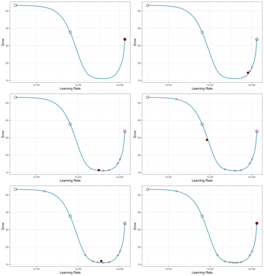
Iterative Search

We could start with a few points and search the space:

Grid Search

Parameters

The tidymodels framework provides pre-defined information on tuning parameters (such as their type, range, transformations, etc).
The extract_parameter_set_dials() function extracts these tuning parameters and the info.

Grids

Create your grid manually or automatically.
The grid_*() functions can make a grid.

Create a grid

lgbm_wflow %>% 
  extract_parameter_set_dials()
#> Collection of 4 parameters for tuning
#> 
#>    identifier       type    object
#>         trees      trees nparam[+]
#>    learn_rate learn_rate nparam[+]
#>    agent hash  num_terms nparam[+]
#>  company hash  num_terms nparam[+]

# Individual functions: 
trees()
#> # Trees (quantitative)
#> Range: [1, 2000]
learn_rate()
#> Learning Rate (quantitative)
#> Transformer: log-10 [1e-100, Inf]
#> Range (transformed scale): [-10, -1]

A parameter set can be updated (e.g. to change the ranges).

Create a grid

set.seed(12)
grid <- 
  lgbm_wflow %>% 
  extract_parameter_set_dials() %>% 
  grid_latin_hypercube(size = 25)

grid
#> # A tibble: 25 × 4
#>    trees    learn_rate `agent hash` `company hash`
#>    <int>         <dbl>        <int>          <int>
#>  1  1629 0.00000440             524           1454
#>  2  1746 0.0000000751          1009           2865
#>  3    53 0.0000180             2313            367
#>  4   442 0.000000445            347            460
#>  5  1413 0.0000000208          3232            553
#>  6  1488 0.0000578             3692            639
#>  7   906 0.000385               602            332
#>  8  1884 0.00000000101         1127            567
#>  9  1812 0.0239                 961           1183
#> 10   393 0.000000117            487           1783
#> # ℹ 15 more rows

A space-filling design tends to perform better than random grids.
Space-filling designs are also usually more efficient than regular grids.

Your turn

Create a grid for our tunable workflow.

Try creating a regular grid.

03:00

Create a regular grid

set.seed(12)
grid <- 
  lgbm_wflow %>% 
  extract_parameter_set_dials() %>% 
  grid_regular(levels = 4)

grid
#> # A tibble: 256 × 4
#>    trees   learn_rate `agent hash` `company hash`
#>    <int>        <dbl>        <int>          <int>
#>  1     1 0.0000000001          256            256
#>  2   667 0.0000000001          256            256
#>  3  1333 0.0000000001          256            256
#>  4  2000 0.0000000001          256            256
#>  5     1 0.0000001             256            256
#>  6   667 0.0000001             256            256
#>  7  1333 0.0000001             256            256
#>  8  2000 0.0000001             256            256
#>  9     1 0.0001                256            256
#> 10   667 0.0001                256            256
#> # ℹ 246 more rows

Your turn

What advantage would a regular grid have?

Update parameter ranges

lgbm_param <- 
  lgbm_wflow %>% 
  extract_parameter_set_dials() %>% 
  update(trees = trees(c(1L, 100L)),
         learn_rate = learn_rate(c(-5, -1)))

set.seed(712)
grid <- 
  lgbm_param %>% 
  grid_latin_hypercube(size = 25)

grid
#> # A tibble: 25 × 4
#>    trees learn_rate `agent hash` `company hash`
#>    <int>      <dbl>        <int>          <int>
#>  1    75  0.000312          2991           1250
#>  2     4  0.0000337          899           3088
#>  3    15  0.0295             520           1578
#>  4     8  0.0997            1256           3592
#>  5    80  0.000622           419            258
#>  6    70  0.000474          2499           1089
#>  7    35  0.000165           287           2376
#>  8    64  0.00137            389            359
#>  9    58  0.0000250          616            881
#> 10    84  0.0639            2311           2635
#> # ℹ 15 more rows

The results

grid %>% 
  ggplot(aes(trees, learn_rate)) +
  geom_point(size = 4) +
  scale_y_log10()

Note that the learning rates are uniform on the log-10 scale.

Use the `tune_*()` functions to tune models

Choosing tuning parameters

Let’s take our previous model and tune more parameters:

lgbm_spec <- 
  boost_tree(trees = tune(), learn_rate = tune(),  min_n = tune()) %>% 
  set_mode("regression") %>% 
  set_engine("lightgbm", num_threads = 1)

lgbm_wflow <- workflow(hash_rec, lgbm_spec)

# Update the feature hash ranges (log-2 units)
lgbm_param <-
  lgbm_wflow %>%
  extract_parameter_set_dials() %>%
  update(`agent hash`   = num_hash(c(3, 8)),
         `company hash` = num_hash(c(3, 8)))

Grid Search

set.seed(9)
ctrl <- control_grid(save_pred = TRUE)

lgbm_res <-
  lgbm_wflow %>%
  tune_grid(
    resamples = hotel_rs,
    grid = 25,
    # The options below are not required by default
    param_info = lgbm_param, 
    control = ctrl,
    metrics = reg_metrics
  )

Grid Search

lgbm_res 
#> # Tuning results
#> # 10-fold cross-validation using stratification 
#> # A tibble: 10 × 5
#>    splits             id     .metrics          .notes           .predictions        
#>    <list>             <chr>  <list>            <list>           <list>              
#>  1 <split [3372/377]> Fold01 <tibble [50 × 9]> <tibble [0 × 3]> <tibble [9,425 × 9]>
#>  2 <split [3373/376]> Fold02 <tibble [50 × 9]> <tibble [0 × 3]> <tibble [9,400 × 9]>
#>  3 <split [3373/376]> Fold03 <tibble [50 × 9]> <tibble [0 × 3]> <tibble [9,400 × 9]>
#>  4 <split [3373/376]> Fold04 <tibble [50 × 9]> <tibble [0 × 3]> <tibble [9,400 × 9]>
#>  5 <split [3373/376]> Fold05 <tibble [50 × 9]> <tibble [0 × 3]> <tibble [9,400 × 9]>
#>  6 <split [3374/375]> Fold06 <tibble [50 × 9]> <tibble [0 × 3]> <tibble [9,375 × 9]>
#>  7 <split [3375/374]> Fold07 <tibble [50 × 9]> <tibble [0 × 3]> <tibble [9,350 × 9]>
#>  8 <split [3376/373]> Fold08 <tibble [50 × 9]> <tibble [0 × 3]> <tibble [9,325 × 9]>
#>  9 <split [3376/373]> Fold09 <tibble [50 × 9]> <tibble [0 × 3]> <tibble [9,325 × 9]>
#> 10 <split [3376/373]> Fold10 <tibble [50 × 9]> <tibble [0 × 3]> <tibble [9,325 × 9]>

Grid results

autoplot(lgbm_res)

Tuning results

collect_metrics(lgbm_res)
#> # A tibble: 50 × 11
#>    trees min_n learn_rate `agent hash` `company hash` .metric .estimator   mean     n std_err .config              
#>    <int> <int>      <dbl>        <int>          <int> <chr>   <chr>       <dbl> <int>   <dbl> <chr>                
#>  1   298    19   4.15e- 9          222             36 mae     standard   53.2      10 0.427   Preprocessor01_Model1
#>  2   298    19   4.15e- 9          222             36 rsq     standard    0.810    10 0.00686 Preprocessor01_Model1
#>  3  1394     5   5.82e- 6           28             21 mae     standard   52.9      10 0.424   Preprocessor02_Model1
#>  4  1394     5   5.82e- 6           28             21 rsq     standard    0.810    10 0.00800 Preprocessor02_Model1
#>  5   774    12   4.41e- 2           27             95 mae     standard    9.77     10 0.155   Preprocessor03_Model1
#>  6   774    12   4.41e- 2           27             95 rsq     standard    0.946    10 0.00341 Preprocessor03_Model1
#>  7  1342     7   6.84e-10           71             17 mae     standard   53.2      10 0.427   Preprocessor04_Model1
#>  8  1342     7   6.84e-10           71             17 rsq     standard    0.811    10 0.00785 Preprocessor04_Model1
#>  9   669    39   8.62e- 7          141            145 mae     standard   53.2      10 0.426   Preprocessor05_Model1
#> 10   669    39   8.62e- 7          141            145 rsq     standard    0.807    10 0.00639 Preprocessor05_Model1
#> # ℹ 40 more rows

Tuning results

collect_metrics(lgbm_res, summarize = FALSE)
#> # A tibble: 500 × 10
#>    id     trees min_n    learn_rate `agent hash` `company hash` .metric .estimator .estimate .config              
#>    <chr>  <int> <int>         <dbl>        <int>          <int> <chr>   <chr>          <dbl> <chr>                
#>  1 Fold01   298    19 0.00000000415          222             36 mae     standard      51.8   Preprocessor01_Model1
#>  2 Fold01   298    19 0.00000000415          222             36 rsq     standard       0.821 Preprocessor01_Model1
#>  3 Fold02   298    19 0.00000000415          222             36 mae     standard      52.1   Preprocessor01_Model1
#>  4 Fold02   298    19 0.00000000415          222             36 rsq     standard       0.804 Preprocessor01_Model1
#>  5 Fold03   298    19 0.00000000415          222             36 mae     standard      52.2   Preprocessor01_Model1
#>  6 Fold03   298    19 0.00000000415          222             36 rsq     standard       0.786 Preprocessor01_Model1
#>  7 Fold04   298    19 0.00000000415          222             36 mae     standard      51.7   Preprocessor01_Model1
#>  8 Fold04   298    19 0.00000000415          222             36 rsq     standard       0.826 Preprocessor01_Model1
#>  9 Fold05   298    19 0.00000000415          222             36 mae     standard      55.2   Preprocessor01_Model1
#> 10 Fold05   298    19 0.00000000415          222             36 rsq     standard       0.845 Preprocessor01_Model1
#> # ℹ 490 more rows

Choose a parameter combination

show_best(lgbm_res, metric = "rsq")
#> # A tibble: 5 × 11
#>   trees min_n learn_rate `agent hash` `company hash` .metric .estimator  mean     n std_err .config              
#>   <int> <int>      <dbl>        <int>          <int> <chr>   <chr>      <dbl> <int>   <dbl> <chr>                
#> 1  1890    10    0.0159           115            174 rsq     standard   0.948    10 0.00334 Preprocessor12_Model1
#> 2   774    12    0.0441            27             95 rsq     standard   0.946    10 0.00341 Preprocessor03_Model1
#> 3  1638    36    0.0409            15            120 rsq     standard   0.945    10 0.00384 Preprocessor16_Model1
#> 4   963    23    0.00556          157             13 rsq     standard   0.937    10 0.00320 Preprocessor06_Model1
#> 5   590     5    0.00320           85             73 rsq     standard   0.908    10 0.00465 Preprocessor24_Model1

Choose a parameter combination

Create your own tibble for final parameters or use one of the tune::select_*() functions:

lgbm_best <- select_best(lgbm_res, metric = "mae")
lgbm_best
#> # A tibble: 1 × 6
#>   trees min_n learn_rate `agent hash` `company hash` .config              
#>   <int> <int>      <dbl>        <int>          <int> <chr>                
#> 1  1890    10     0.0159          115            174 Preprocessor12_Model1

Checking Calibration

library(probably)
lgbm_res %>%
  collect_predictions(
    parameters = lgbm_best
  ) %>%
  cal_plot_regression(
    truth = avg_price_per_room,
    estimate = .pred,
    alpha = 1 / 3
  )

Running in parallel

Grid search, combined with resampling, requires fitting a lot of models!
These models don’t depend on one another and can be run in parallel.

We can use a parallel backend to do this:

cores <- parallelly::availableCores(logical = FALSE)
cl <- parallel::makePSOCKcluster(cores)
doParallel::registerDoParallel(cl)

# Now call `tune_grid()`!

# Shut it down with:
foreach::registerDoSEQ()
parallel::stopCluster(cl)

Running in parallel

Speed-ups are fairly linear up to the number of physical cores (10 here).

Early stopping for boosted trees

We have directly optimized the number of trees as a tuning parameter.

Instead we could

Set the number of trees to a single large number.
Stop adding trees when performance gets worse.

This is known as “early stopping” and there is a parameter for that: stop_iter.

Early stopping has a potential to decrease the tuning time.

Your turn

Set trees = 2000 and tune the stop_iter parameter.

Note that you will need to regenerate lgbm_param with your new workflow!

10:00

2 - Tuning Hyperparameters

Previously - Setup

Previously - Data Usage

Previously - Feature engineering

Optimizing Models via Tuning Parameters

Tuning parameters

Activation function in neural networks?

Number of feature hashing columns to generate?

Bayesian priors for model parameters?

Covariance/correlation matrix structure in mixed models?

Is the random seed a tuning parameter?

Optimize tuning parameters

Tagging parameters for tuning

Optimizing the hash features

Boosted Trees

Boosted Tree Tuning Parameters

Boosted Tree Tuning Parameters

Boosted Tree Tuning Parameters

Optimize tuning parameters

Grid search

Grid search

Iterative Search

Grid Search

Parameters

Grids

Create a grid

Create a grid

Your turn

Create a regular grid

Your turn

Update parameter ranges

The results

Use the tune_*() functions to tune models

Choosing tuning parameters

Grid Search

Grid Search

Grid results

Tuning results

Tuning results

Choose a parameter combination

Choose a parameter combination

Checking Calibration

Running in parallel

Running in parallel

Early stopping for boosted trees

Your turn

Use the `tune_*()` functions to tune models