2 - Your data budget

Machine learning with tidymodels

Data on Chicago taxi trips

• The city of Chicago releases anonymized trip-level data on taxi trips in the city.
• We pulled a sample of 10,000 rides occurring in early 2022.
• Type ?modeldatatoo::data_taxi() to learn more about this dataset, including references.

Which of these variables can we use?

library(tidymodels)
library(modeldatatoo)

taxi <- data_taxi()

names(taxi)
#>  [1] "tip"          "id"           "duration"     "distance"     "fare"        
#>  [6] "tolls"        "extras"       "total_cost"   "payment_type" "company"     
#> [11] "local"        "dow"          "month"        "hour"

Checklist for predictors

• Is it ethical to use this variable? (Or even legal?)

• Will this variable be available at prediction time?

• Does this variable contribute to explainability?

Data on Chicago taxi trips

We are using a slightly modified version from the modeldatatoo data.

taxi <- taxi %>%
  mutate(month = factor(month, levels = c("Jan", "Feb", "Mar", "Apr"))) %>% 
  select(-c(id, duration, fare, tolls, extras, total_cost, payment_type)) %>% 
  drop_na()

Data on Chicago taxi trips

• N = 10,000
• A nominal outcome, tip, with levels "yes" and "no"
• 6 other variables
  • company, local, and dow, and month are nominal predictors
  • distance and hours are numeric predictors

tip: Whether the rider left a tip. A factor with levels “yes” and “no”.

distance: The trip distance, in odometer miles.

company: The taxi company, as a factor. Companies that occurred few times were binned as “other”.

local: Whether the trip started in the same community area as it began. See the source data for community area values.

dow: The day of the week in which the trip began, as a factor.

month: The month in which the trip began, as a factor.

hour: The hour of the day in which the trip began, as a numeric.

Data on Chicago taxi trips

taxi
#> # A tibble: 8,807 × 7
#>    tip   distance company      local dow   month  hour
#>    <fct>    <dbl> <fct>        <fct> <fct> <fct> <int>
#>  1 yes       1.24 Sun Taxi     no    Thu   Feb      13
#>  2 no        5.39 Flash Cab    no    Sat   Mar      12
#>  3 yes       3.01 City Service no    Wed   Feb      17
#>  4 no       18.4  Sun Taxi     no    Sat   Apr       6
#>  5 yes       1.76 Sun Taxi     no    Sun   Jan      15
#>  6 yes      13.6  Sun Taxi     no    Mon   Feb      17
#>  7 yes       3.71 City Service no    Mon   Mar      21
#>  8 yes       4.8  other        no    Tue   Mar       9
#>  9 yes      18.0  City Service no    Fri   Jan      19
#> 10 no       17.5  other        yes   Thu   Apr      12
#> # ℹ 8,797 more rows

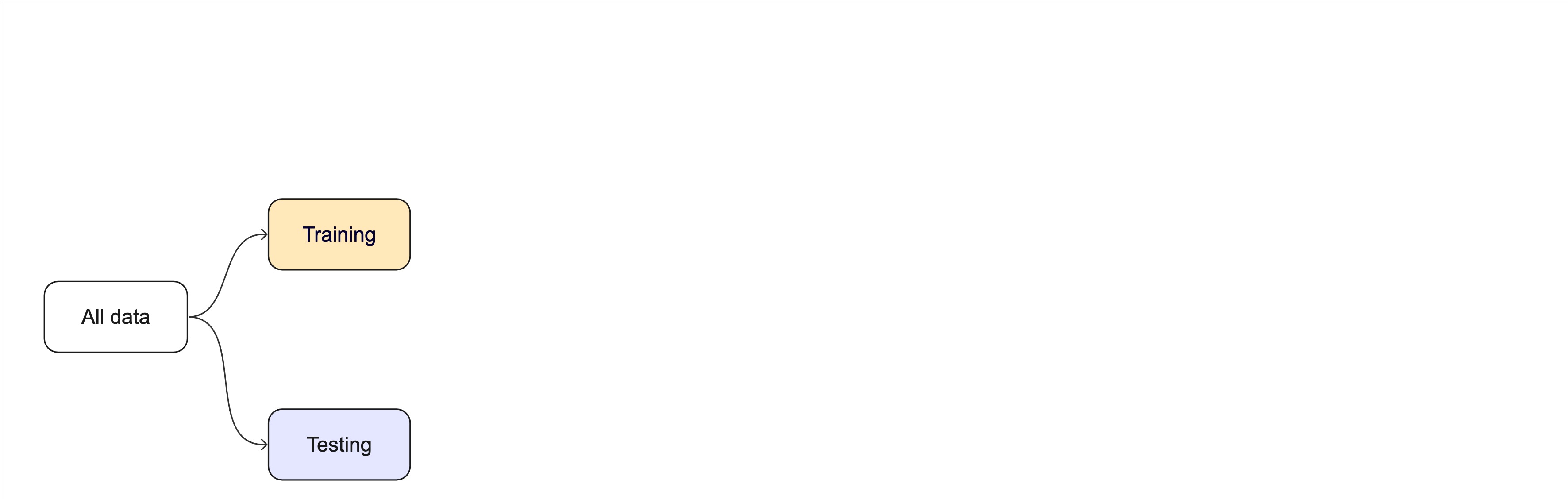
Data splitting and spending

For machine learning, we typically split data into training and test sets:

• The training set is used to estimate model parameters.
• The test set is used to find an independent assessment of model performance.

Do not 🚫 use the test set during training.

Data splitting and spending

The more data
we spend 🤑

the better estimates
we’ll get.

Data splitting and spending

• Spending too much data in training prevents us from computing a good assessment of predictive performance.

• Spending too much data in testing prevents us from computing a good estimate of model parameters.

Your turn

When is a good time to split your data?

03:00

The testing data is precious 💎

The initial split

set.seed(123)
taxi_split <- initial_split(taxi)
taxi_split
#> <Training/Testing/Total>
#> <6605/2202/8807>

How much data in training vs testing? This function uses a good default, but this depends on your specific goal/data We will talk about more powerful ways of splitting, like stratification, later

Accessing the data

taxi_train <- training(taxi_split)
taxi_test <- testing(taxi_split)

The training set

taxi_train
#> # A tibble: 6,605 × 7
#>    tip   distance company                   local dow   month  hour
#>    <fct>    <dbl> <fct>                     <fct> <fct> <fct> <int>
#>  1 yes       4.54 City Service              no    Sat   Mar      16
#>  2 no       10.2  Flash Cab                 no    Mon   Feb       8
#>  3 yes      12.4  other                     no    Sun   Apr      15
#>  4 yes      15.3  Sun Taxi                  no    Mon   Apr      18
#>  5 no        6.41 Flash Cab                 no    Wed   Apr      14
#>  6 yes       1.56 other                     no    Tue   Jan      13
#>  7 yes       3.13 Flash Cab                 no    Sun   Apr      12
#>  8 yes       7.54 other                     no    Tue   Apr       8
#>  9 yes       6.98 Flash Cab                 no    Tue   Apr       5
#> 10 yes       0.7  Taxi Affiliation Services no    Tue   Jan       9
#> # ℹ 6,595 more rows

The test set

🙈

There are 2202 rows and 7 columns in the test set.

Your turn

Split your data so 20% is held out for the test set.

Try out different values in set.seed() to see how the results change.

05:00

Data splitting and spending

set.seed(123)
taxi_split <- initial_split(taxi, prop = 0.8)
taxi_train <- training(taxi_split)
taxi_test <- testing(taxi_split)

nrow(taxi_train)
#> [1] 7045
nrow(taxi_test)
#> [1] 1762

What about a validation set?

We will use this tomorrow

Exploratory data analysis for ML 🧐

Your turn

Explore the taxi_train data on your own!

• What’s the distribution of the outcome, tip?
• What’s the distribution of numeric variables like distance?
• How does tip differ across the categorical variables?

08:00

Make a plot or summary and then share with neighbor

taxi_train %>% 
  ggplot(aes(x = tip)) +
  geom_bar()

taxi_train %>% 
  ggplot(aes(x = tip, fill = local)) +
  geom_bar() +
  scale_fill_viridis_d(end = .5)

taxi_train %>% 
  mutate(tip = forcats::fct_rev(tip)) %>% 
  ggplot(aes(x = hour, fill = tip)) +
  geom_bar()

taxi_train %>% 
  mutate(tip = forcats::fct_rev(tip)) %>% 
  ggplot(aes(x = hour, fill = tip)) +
  geom_bar(position = "fill")

taxi_train %>% 
  mutate(tip = forcats::fct_rev(tip)) %>% 
  ggplot(aes(x = distance)) +
  geom_histogram(bins = 100) +
  facet_grid(vars(tip))

Split smarter

Stratified sampling would split within response values

Based on our EDA, we know that the source data contains fewer "no" tip values than "yes". We want to make sure we allot equal proportions of those responses so that both the training and testing data have enough of each to give accurate estimates.

Stratification

Use strata = tip

set.seed(123)
taxi_split <- initial_split(taxi, prop = 0.8, strata = tip)
taxi_split
#> <Training/Testing/Total>
#> <7045/1762/8807>

Stratification

Stratification often helps, with very little downside

The whole game - status update