4 - Evaluating models

Machine learning with tidymodels

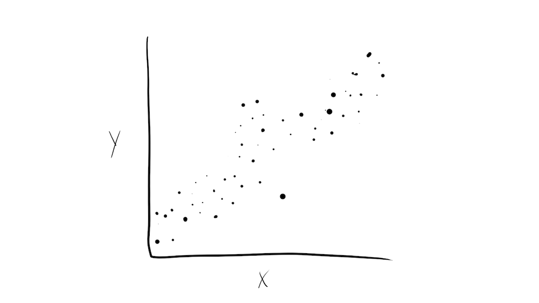
Metrics for model performance

augment(tree_fit, new_data = frog_test) %>%
  metrics(latency, .pred)
#> # A tibble: 3 × 3
#>   .metric .estimator .estimate
#>   <chr>   <chr>          <dbl>
#> 1 rmse    standard      59.2  
#> 2 rsq     standard       0.380
#> 3 mae     standard      40.2

• RMSE: difference between the predicted and observed values ⬇️
• \(R^2\): squared correlation between the predicted and observed values ⬆️
• MAE: similar to RMSE, but mean absolute error ⬇️

Metrics for model performance

augment(tree_fit, new_data = frog_test) %>%
  rmse(latency, .pred)
#> # A tibble: 1 × 3
#>   .metric .estimator .estimate
#>   <chr>   <chr>          <dbl>
#> 1 rmse    standard        59.2

Metrics for model performance

augment(tree_fit, new_data = frog_test) %>%
  group_by(reflex) %>%
  rmse(latency, .pred)
#> # A tibble: 3 × 4
#>   reflex .metric .estimator .estimate
#>   <fct>  <chr>   <chr>          <dbl>
#> 1 low    rmse    standard        94.3
#> 2 mid    rmse    standard       101. 
#> 3 full   rmse    standard        51.2

Metrics for model performance

frog_metrics <- metric_set(rmse, msd)
augment(tree_fit, new_data = frog_test) %>%
  frog_metrics(latency, .pred)
#> # A tibble: 2 × 3
#>   .metric .estimator .estimate
#>   <chr>   <chr>          <dbl>
#> 1 rmse    standard      59.2  
#> 2 msd     standard      -0.908

We’ll talk about classification metrics tomorrow!

⚠️ DANGERS OF OVERFITTING ⚠️

Dangers of overfitting ⚠️

Dangers of overfitting ⚠️

Dangers of overfitting ⚠️

tree_fit %>%
  augment(frog_train)
#> # A tibble: 456 × 6
#>    treatment  reflex   age t_o_d     latency .pred
#>    <chr>      <fct>  <dbl> <fct>       <dbl> <dbl>
#>  1 control    full    5.42 morning        33  39.8
#>  2 control    full    5.38 morning        19  66.7
#>  3 control    full    5.38 morning         2  66.7
#>  4 control    full    5.44 morning        39  39.8
#>  5 control    full    5.41 morning        42  39.8
#>  6 control    full    4.75 afternoon      20  59.8
#>  7 control    full    4.95 night          31  83.1
#>  8 control    full    5.42 morning        21  39.8
#>  9 gentamicin full    5.39 morning        30  64.6
#> 10 control    full    4.55 afternoon      43 174. 
#> # … with 446 more rows
#> # ℹ Use `print(n = ...)` to see more rows

We call this “resubstitution” or “repredicting the training set”

Dangers of overfitting ⚠️

tree_fit %>%
  augment(frog_train) %>%
  rmse(latency, .pred)
#> # A tibble: 1 × 3
#>   .metric .estimator .estimate
#>   <chr>   <chr>          <dbl>
#> 1 rmse    standard        49.4

We call this a “resubstitution estimate”

Dangers of overfitting ⚠️

tree_fit %>%
  augment(frog_train) %>%
  rmse(latency, .pred)
#> # A tibble: 1 × 3
#>   .metric .estimator .estimate
#>   <chr>   <chr>          <dbl>
#> 1 rmse    standard        49.4

Dangers of overfitting ⚠️

tree_fit %>%
  augment(frog_train) %>%
  rmse(latency, .pred)
#> # A tibble: 1 × 3
#>   .metric .estimator .estimate
#>   <chr>   <chr>          <dbl>
#> 1 rmse    standard        49.4

tree_fit %>%
  augment(frog_test) %>%
  rmse(latency, .pred)
#> # A tibble: 1 × 3
#>   .metric .estimator .estimate
#>   <chr>   <chr>          <dbl>
#> 1 rmse    standard        59.2

⚠️ Remember that we’re demonstrating overfitting

⚠️ Don’t use the test set until the end of your modeling analysis

Your turn

Use augment() and metrics() to compute a regression metric like mae().

Compute the metrics for both training and testing data.

Notice the evidence of overfitting! ⚠️

05:00

Dangers of overfitting ⚠️

tree_fit %>%
  augment(frog_train) %>%
  metrics(latency, .pred)
#> # A tibble: 3 × 3
#>   .metric .estimator .estimate
#>   <chr>   <chr>          <dbl>
#> 1 rmse    standard      49.4  
#> 2 rsq     standard       0.494
#> 3 mae     standard      33.4

tree_fit %>%
  augment(frog_test) %>%
  metrics(latency, .pred)
#> # A tibble: 3 × 3
#>   .metric .estimator .estimate
#>   <chr>   <chr>          <dbl>
#> 1 rmse    standard      59.2  
#> 2 rsq     standard       0.380
#> 3 mae     standard      40.2

What if we want to compare more models?

And/or more model configurations?

And we want to understand if these are important differences?

The testing data are precious 💎

How can we use the training data to compare and evaluate different models? 🤔

Cross-validation

Cross-validation

Your turn

If we use 10 folds, what percent of the training data

• ends up in analysis
• ends up in assessment

for each fold?

03:00

Cross-validation

vfold_cv(frog_train) # v = 10 is default
#> #  10-fold cross-validation 
#> # A tibble: 10 × 2
#>    splits           id    
#>    <list>           <chr> 
#>  1 <split [410/46]> Fold01
#>  2 <split [410/46]> Fold02
#>  3 <split [410/46]> Fold03
#>  4 <split [410/46]> Fold04
#>  5 <split [410/46]> Fold05
#>  6 <split [410/46]> Fold06
#>  7 <split [411/45]> Fold07
#>  8 <split [411/45]> Fold08
#>  9 <split [411/45]> Fold09
#> 10 <split [411/45]> Fold10

Cross-validation

What is in this?

frog_folds <- vfold_cv(frog_train)
frog_folds$splits[1:3]
#> [[1]]
#> <Analysis/Assess/Total>
#> <410/46/456>
#> 
#> [[2]]
#> <Analysis/Assess/Total>
#> <410/46/456>
#> 
#> [[3]]
#> <Analysis/Assess/Total>
#> <410/46/456>

Talk about a list column, storing non-atomic types in dataframe

Cross-validation

vfold_cv(frog_train, v = 5)
#> #  5-fold cross-validation 
#> # A tibble: 5 × 2
#>   splits           id   
#>   <list>           <chr>
#> 1 <split [364/92]> Fold1
#> 2 <split [365/91]> Fold2
#> 3 <split [365/91]> Fold3
#> 4 <split [365/91]> Fold4
#> 5 <split [365/91]> Fold5

Cross-validation

vfold_cv(frog_train, strata = latency)
#> #  10-fold cross-validation using stratification 
#> # A tibble: 10 × 2
#>    splits           id    
#>    <list>           <chr> 
#>  1 <split [408/48]> Fold01
#>  2 <split [408/48]> Fold02
#>  3 <split [408/48]> Fold03
#>  4 <split [409/47]> Fold04
#>  5 <split [411/45]> Fold05
#>  6 <split [412/44]> Fold06
#>  7 <split [412/44]> Fold07
#>  8 <split [412/44]> Fold08
#>  9 <split [412/44]> Fold09
#> 10 <split [412/44]> Fold10

Stratification often helps, with very little downside

Cross-validation

We’ll use this setup:

set.seed(123)
frog_folds <- vfold_cv(frog_train, v = 10, strata = latency)
frog_folds
#> #  10-fold cross-validation using stratification 
#> # A tibble: 10 × 2
#>    splits           id    
#>    <list>           <chr> 
#>  1 <split [408/48]> Fold01
#>  2 <split [408/48]> Fold02
#>  3 <split [408/48]> Fold03
#>  4 <split [409/47]> Fold04
#>  5 <split [411/45]> Fold05
#>  6 <split [412/44]> Fold06
#>  7 <split [412/44]> Fold07
#>  8 <split [412/44]> Fold08
#>  9 <split [412/44]> Fold09
#> 10 <split [412/44]> Fold10

Set the seed when creating resamples

We are equipped with metrics and resamples!

Fit our model to the resamples

tree_res <- fit_resamples(tree_wflow, frog_folds)
tree_res
#> # Resampling results
#> # 10-fold cross-validation using stratification 
#> # A tibble: 10 × 4
#>    splits           id     .metrics         .notes          
#>    <list>           <chr>  <list>           <list>          
#>  1 <split [408/48]> Fold01 <tibble [2 × 4]> <tibble [0 × 3]>
#>  2 <split [408/48]> Fold02 <tibble [2 × 4]> <tibble [0 × 3]>
#>  3 <split [408/48]> Fold03 <tibble [2 × 4]> <tibble [0 × 3]>
#>  4 <split [409/47]> Fold04 <tibble [2 × 4]> <tibble [0 × 3]>
#>  5 <split [411/45]> Fold05 <tibble [2 × 4]> <tibble [0 × 3]>
#>  6 <split [412/44]> Fold06 <tibble [2 × 4]> <tibble [0 × 3]>
#>  7 <split [412/44]> Fold07 <tibble [2 × 4]> <tibble [0 × 3]>
#>  8 <split [412/44]> Fold08 <tibble [2 × 4]> <tibble [0 × 3]>
#>  9 <split [412/44]> Fold09 <tibble [2 × 4]> <tibble [0 × 3]>
#> 10 <split [412/44]> Fold10 <tibble [2 × 4]> <tibble [0 × 3]>

Evaluating model performance

tree_res %>%
  collect_metrics()
#> # A tibble: 2 × 6
#>   .metric .estimator   mean     n std_err .config             
#>   <chr>   <chr>       <dbl> <int>   <dbl> <chr>               
#> 1 rmse    standard   59.6      10  2.31   Preprocessor1_Model1
#> 2 rsq     standard    0.305    10  0.0342 Preprocessor1_Model1

We can reliably measure performance using only the training data 🎉

Comparing metrics

How do the metrics from resampling compare to the metrics from training and testing?

tree_res %>%
  collect_metrics() %>% 
  select(.metric, mean, n)
#> # A tibble: 2 × 3
#>   .metric   mean     n
#>   <chr>    <dbl> <int>
#> 1 rmse    59.6      10
#> 2 rsq      0.305    10

The RMSE previously was

• 49.36 for the training set
• 59.16 for test set

Remember that:

⚠️ the training set gives you overly optimistic metrics

⚠️ the test set is precious

Evaluating model performance

# Save the assessment set results
ctrl_frog <- control_resamples(save_pred = TRUE)
tree_res <- fit_resamples(tree_wflow, frog_folds, control = ctrl_frog)

tree_preds <- collect_predictions(tree_res)
tree_preds
#> # A tibble: 456 × 5
#>    id     .pred  .row latency .config             
#>    <chr>  <dbl> <int>   <dbl> <chr>               
#>  1 Fold01  39.6     1      33 Preprocessor1_Model1
#>  2 Fold01  72.1     3       2 Preprocessor1_Model1
#>  3 Fold01  63.8     9      30 Preprocessor1_Model1
#>  4 Fold01  72.1    13      46 Preprocessor1_Model1
#>  5 Fold01  43.3    28      11 Preprocessor1_Model1
#>  6 Fold01  61.7    35      41 Preprocessor1_Model1
#>  7 Fold01  39.6    51      43 Preprocessor1_Model1
#>  8 Fold01 134.     70      20 Preprocessor1_Model1
#>  9 Fold01  70.6    74      21 Preprocessor1_Model1
#> 10 Fold01  39.6   106      14 Preprocessor1_Model1
#> # … with 446 more rows
#> # ℹ Use `print(n = ...)` to see more rows

tree_preds %>% 
  ggplot(aes(latency, .pred, color = id)) + 
  geom_abline(lty = 2, col = "gray", size = 1.5) +
  geom_point(alpha = 0.5) +
  coord_obs_pred()

Where are the fitted models?

tree_res
#> # Resampling results
#> # 10-fold cross-validation using stratification 
#> # A tibble: 10 × 5
#>    splits           id     .metrics         .notes           .predictions     
#>    <list>           <chr>  <list>           <list>           <list>           
#>  1 <split [408/48]> Fold01 <tibble [2 × 4]> <tibble [0 × 3]> <tibble [48 × 4]>
#>  2 <split [408/48]> Fold02 <tibble [2 × 4]> <tibble [0 × 3]> <tibble [48 × 4]>
#>  3 <split [408/48]> Fold03 <tibble [2 × 4]> <tibble [0 × 3]> <tibble [48 × 4]>
#>  4 <split [409/47]> Fold04 <tibble [2 × 4]> <tibble [0 × 3]> <tibble [47 × 4]>
#>  5 <split [411/45]> Fold05 <tibble [2 × 4]> <tibble [0 × 3]> <tibble [45 × 4]>
#>  6 <split [412/44]> Fold06 <tibble [2 × 4]> <tibble [0 × 3]> <tibble [44 × 4]>
#>  7 <split [412/44]> Fold07 <tibble [2 × 4]> <tibble [0 × 3]> <tibble [44 × 4]>
#>  8 <split [412/44]> Fold08 <tibble [2 × 4]> <tibble [0 × 3]> <tibble [44 × 4]>
#>  9 <split [412/44]> Fold09 <tibble [2 × 4]> <tibble [0 × 3]> <tibble [44 × 4]>
#> 10 <split [412/44]> Fold10 <tibble [2 × 4]> <tibble [0 × 3]> <tibble [44 × 4]>

🗑️

Alternate resampling schemes

Bootstrapping

Bootstrapping

set.seed(3214)
bootstraps(frog_train)
#> # Bootstrap sampling 
#> # A tibble: 25 × 2
#>    splits            id         
#>    <list>            <chr>      
#>  1 <split [456/163]> Bootstrap01
#>  2 <split [456/166]> Bootstrap02
#>  3 <split [456/173]> Bootstrap03
#>  4 <split [456/177]> Bootstrap04
#>  5 <split [456/166]> Bootstrap05
#>  6 <split [456/163]> Bootstrap06
#>  7 <split [456/164]> Bootstrap07
#>  8 <split [456/165]> Bootstrap08
#>  9 <split [456/170]> Bootstrap09
#> 10 <split [456/177]> Bootstrap10
#> # … with 15 more rows
#> # ℹ Use `print(n = ...)` to see more rows

Your turn

Create:

• bootstrap folds (change times from the default)
• validation set (use the reference guide to find the function)

Don’t forget to set a seed when you resample!

05:00

Bootstrapping

set.seed(322)
bootstraps(frog_train, times = 10)
#> # Bootstrap sampling 
#> # A tibble: 10 × 2
#>    splits            id         
#>    <list>            <chr>      
#>  1 <split [456/173]> Bootstrap01
#>  2 <split [456/168]> Bootstrap02
#>  3 <split [456/170]> Bootstrap03
#>  4 <split [456/164]> Bootstrap04
#>  5 <split [456/176]> Bootstrap05
#>  6 <split [456/156]> Bootstrap06
#>  7 <split [456/166]> Bootstrap07
#>  8 <split [456/168]> Bootstrap08
#>  9 <split [456/167]> Bootstrap09
#> 10 <split [456/170]> Bootstrap10

Validation set

set.seed(853)
validation_split(frog_train, strata = latency)
#> # Validation Set Split (0.75/0.25)  using stratification 
#> # A tibble: 1 × 2
#>   splits            id        
#>   <list>            <chr>     
#> 1 <split [340/116]> validation

A validation set is just another type of resample

Decision tree 🌳

Random forest 🌳🌲🌴🌵🌴🌳🌳🌴🌲🌵🌴🌲🌳🌴🌳🌵🌵🌴🌲🌲🌳🌴🌳🌴🌲🌴🌵🌴🌲🌴🌵🌲🌵🌴🌲🌳🌴🌵🌳🌴🌳

Random forest 🌳🌲🌴🌵🌳🌳🌴🌲🌵🌴🌳🌵

• Ensemble many decision tree models

• All the trees vote! 🗳️

• Bootstrap aggregating + random predictor sampling

• Often works well without tuning hyperparameters (more on this tomorrow!), as long as there are enough trees

Create a random forest model

rf_spec <- rand_forest(trees = 1000, mode = "regression")
rf_spec
#> Random Forest Model Specification (regression)
#> 
#> Main Arguments:
#>   trees = 1000
#> 
#> Computational engine: ranger

Create a random forest model

rf_wflow <- workflow(latency ~ ., rf_spec)
rf_wflow
#> ══ Workflow ══════════════════════════════════════════════════════════
#> Preprocessor: Formula
#> Model: rand_forest()
#> 
#> ── Preprocessor ──────────────────────────────────────────────────────
#> latency ~ .
#> 
#> ── Model ─────────────────────────────────────────────────────────────
#> Random Forest Model Specification (regression)
#> 
#> Main Arguments:
#>   trees = 1000
#> 
#> Computational engine: ranger

Your turn

Use fit_resamples() and rf_wflow to:

• keep predictions
• compute metrics
• plot true vs. predicted values

08:00

Evaluating model performance

ctrl_frog <- control_resamples(save_pred = TRUE)

# Random forest uses random numbers so set the seed first

set.seed(2)
rf_res <- fit_resamples(rf_wflow, frog_folds, control = ctrl_frog)
collect_metrics(rf_res)
#> # A tibble: 2 × 6
#>   .metric .estimator   mean     n std_err .config             
#>   <chr>   <chr>       <dbl> <int>   <dbl> <chr>               
#> 1 rmse    standard   55.9      10  1.71   Preprocessor1_Model1
#> 2 rsq     standard    0.370    10  0.0306 Preprocessor1_Model1

collect_predictions(rf_res) %>% 
  ggplot(aes(latency, .pred, color = id)) + 
  geom_abline(lty = 2, col = "gray", size = 1.5) +
  geom_point(alpha = 0.5) +
  coord_obs_pred()

How can we compare multiple model workflows at once?

Evaluate a workflow set

workflow_set(list(latency ~ .), list(tree_spec, rf_spec))
#> # A workflow set/tibble: 2 × 4
#>   wflow_id              info             option    result    
#>   <chr>                 <list>           <list>    <list>    
#> 1 formula_decision_tree <tibble [1 × 4]> <opts[0]> <list [0]>
#> 2 formula_rand_forest   <tibble [1 × 4]> <opts[0]> <list [0]>

Evaluate a workflow set

workflow_set(list(latency ~ .), list(tree_spec, rf_spec)) %>%
  workflow_map("fit_resamples", resamples = frog_folds)
#> # A workflow set/tibble: 2 × 4
#>   wflow_id              info             option    result   
#>   <chr>                 <list>           <list>    <list>   
#> 1 formula_decision_tree <tibble [1 × 4]> <opts[1]> <rsmp[+]>
#> 2 formula_rand_forest   <tibble [1 × 4]> <opts[1]> <rsmp[+]>

Evaluate a workflow set

workflow_set(list(latency ~ .), list(tree_spec, rf_spec)) %>%
  workflow_map("fit_resamples", resamples = frog_folds) %>%
  rank_results()
#> # A tibble: 4 × 9
#>   wflow_id              .config .metric   mean std_err     n prepr…¹ model  rank
#>   <chr>                 <chr>   <chr>    <dbl>   <dbl> <int> <chr>   <chr> <int>
#> 1 formula_rand_forest   Prepro… rmse    55.8    1.71      10 formula rand…     1
#> 2 formula_rand_forest   Prepro… rsq      0.371  0.0301    10 formula rand…     1
#> 3 formula_decision_tree Prepro… rmse    59.6    2.31      10 formula deci…     2
#> 4 formula_decision_tree Prepro… rsq      0.305  0.0342    10 formula deci…     2
#> # … with abbreviated variable name ¹​preprocessor

The first metric of the metric set is used for ranking. Use rank_metric to change that.

Lots more available with workflow sets, like collect_metrics(), autoplot() methods, and more!

Your turn

When do you think a workflow set would be useful?

03:00

The final fit

Suppose that we are happy with our random forest model.

Let’s fit the model on the training set and verify our performance using the test set.

We’ve shown you fit() and predict() (+ augment()) but there is a shortcut:

# frog_split has train + test info
final_fit <- last_fit(rf_wflow, frog_split) 

final_fit
#> # Resampling results
#> # Manual resampling 
#> # A tibble: 1 × 6
#>   splits            id               .metrics .notes   .predictions .workflow 
#>   <list>            <chr>            <list>   <list>   <list>       <list>    
#> 1 <split [456/116]> train/test split <tibble> <tibble> <tibble>     <workflow>

What is in final_fit?

collect_metrics(final_fit)
#> # A tibble: 2 × 4
#>   .metric .estimator .estimate .config             
#>   <chr>   <chr>          <dbl> <chr>               
#> 1 rmse    standard      57.1   Preprocessor1_Model1
#> 2 rsq     standard       0.420 Preprocessor1_Model1

These are metrics computed with the test set

What is in final_fit?

collect_predictions(final_fit)
#> # A tibble: 116 × 5
#>    id               .pred  .row latency .config             
#>    <chr>            <dbl> <int>   <dbl> <chr>               
#>  1 train/test split  43.5     1      22 Preprocessor1_Model1
#>  2 train/test split 104.      3     106 Preprocessor1_Model1
#>  3 train/test split  76.2     6      39 Preprocessor1_Model1
#>  4 train/test split  42.4     8      50 Preprocessor1_Model1
#>  5 train/test split  43.5    10      63 Preprocessor1_Model1
#>  6 train/test split  43.1    14      25 Preprocessor1_Model1
#>  7 train/test split  51.5    16      48 Preprocessor1_Model1
#>  8 train/test split 160.     17      91 Preprocessor1_Model1
#>  9 train/test split  50.9    32      11 Preprocessor1_Model1
#> 10 train/test split 171.     33     109 Preprocessor1_Model1
#> # … with 106 more rows
#> # ℹ Use `print(n = ...)` to see more rows

These are predictions for the test set

collect_predictions(final_fit) %>%
  ggplot(aes(latency, .pred)) + 
  geom_abline(lty = 2, col = "deeppink4", size = 1.5) +
  geom_point(alpha = 0.5) +
  coord_obs_pred()

What is in final_fit?

extract_workflow(final_fit)
#> ══ Workflow [trained] ════════════════════════════════════════════════
#> Preprocessor: Formula
#> Model: rand_forest()
#> 
#> ── Preprocessor ──────────────────────────────────────────────────────
#> latency ~ .
#> 
#> ── Model ─────────────────────────────────────────────────────────────
#> Ranger result
#> 
#> Call:
#>  ranger::ranger(x = maybe_data_frame(x), y = y, num.trees = ~1000,      num.threads = 1, verbose = FALSE, seed = sample.int(10^5,          1)) 
#> 
#> Type:                             Regression 
#> Number of trees:                  1000 
#> Sample size:                      456 
#> Number of independent variables:  4 
#> Mtry:                             2 
#> Target node size:                 5 
#> Variable importance mode:         none 
#> Splitrule:                        variance 
#> OOB prediction error (MSE):       3124.583 
#> R squared (OOB):                  0.3531813

Use this for prediction on new data, like for deploying

Your turn

End of the day discussion!

Which model do you think you would decide to use?

What surprised you the most?

What is one thing you are looking forward to for tomorrow?

05:00

Why choose just one final_fit?

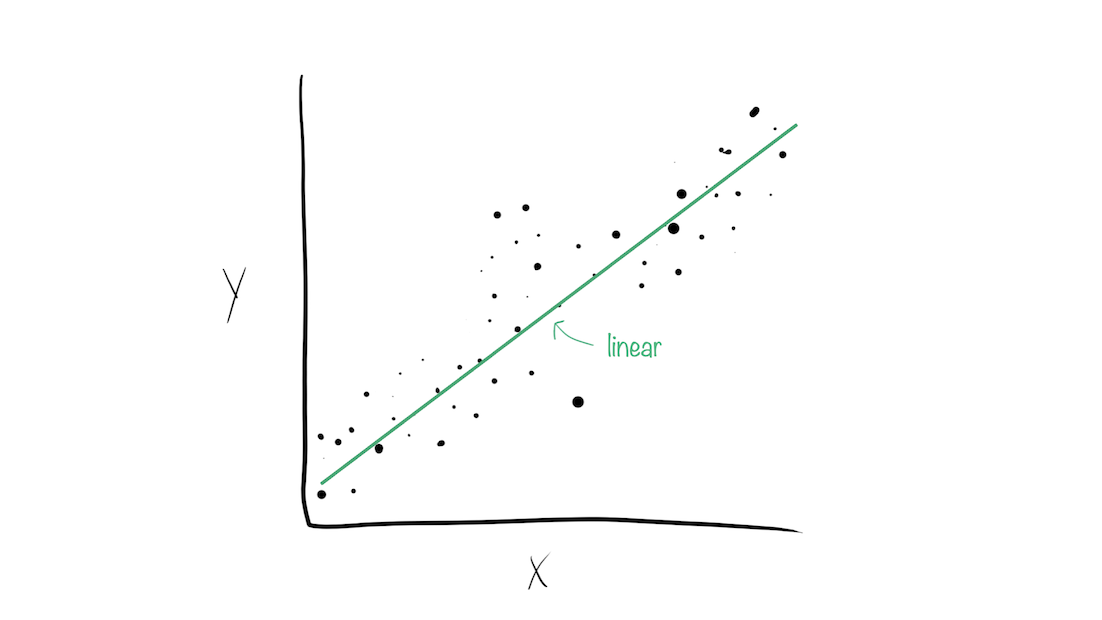
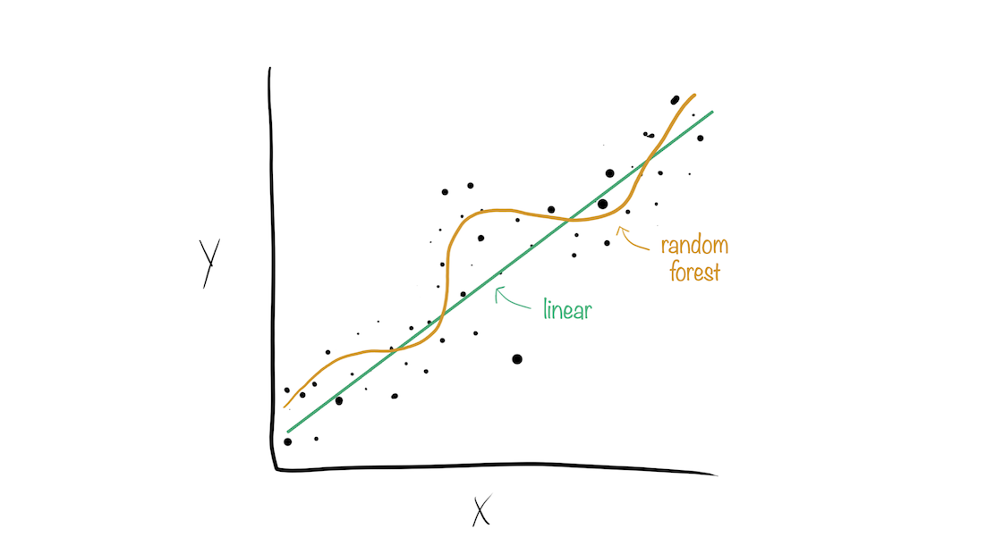
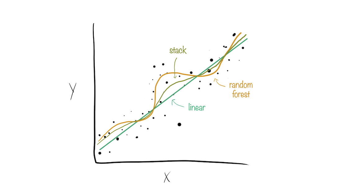
Model stacks generate predictions that are informed by several models.

Why choose just one final_fit?

Why choose just one final_fit?

Why choose just one final_fit?

Why choose just one final_fit?

Why choose just one final_fit?

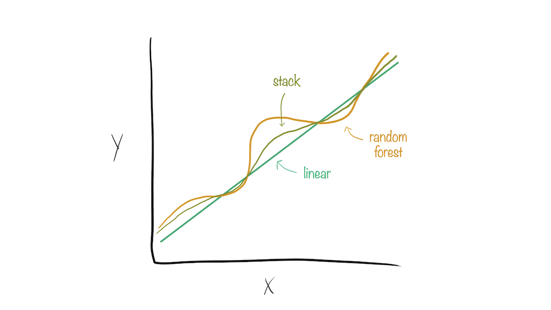
Building a model stack

library(stacks)

1. Define candidate members
2. Initialize a data stack object
3. Iteratively add candidate ensemble members to the data stack
4. Evaluate how to combine their predictions
5. Fit candidate ensemble members with non-zero stacking coefficients
6. Predict on new data!

Building a model stack

stack_ctrl <- control_resamples(save_pred = TRUE, save_workflow = TRUE)

Building a model stack

1. Define candidate members

Start out with a linear regression:

lr_res <- 
  # define model spec
  linear_reg() %>%
  set_mode("regression") %>%
  # add to workflow
  workflow(preprocessor = latency ~ .) %>%
  # fit to resamples
  fit_resamples(frog_folds, control = stack_ctrl)

Building a model stack

lr_res
#> # Resampling results
#> # 10-fold cross-validation using stratification 
#> # A tibble: 10 × 5
#>    splits           id     .metrics         .notes           .predictions     
#>    <list>           <chr>  <list>           <list>           <list>           
#>  1 <split [408/48]> Fold01 <tibble [2 × 4]> <tibble [0 × 3]> <tibble [48 × 4]>
#>  2 <split [408/48]> Fold02 <tibble [2 × 4]> <tibble [0 × 3]> <tibble [48 × 4]>
#>  3 <split [408/48]> Fold03 <tibble [2 × 4]> <tibble [0 × 3]> <tibble [48 × 4]>
#>  4 <split [409/47]> Fold04 <tibble [2 × 4]> <tibble [0 × 3]> <tibble [47 × 4]>
#>  5 <split [411/45]> Fold05 <tibble [2 × 4]> <tibble [0 × 3]> <tibble [45 × 4]>
#>  6 <split [412/44]> Fold06 <tibble [2 × 4]> <tibble [0 × 3]> <tibble [44 × 4]>
#>  7 <split [412/44]> Fold07 <tibble [2 × 4]> <tibble [0 × 3]> <tibble [44 × 4]>
#>  8 <split [412/44]> Fold08 <tibble [2 × 4]> <tibble [0 × 3]> <tibble [44 × 4]>
#>  9 <split [412/44]> Fold09 <tibble [2 × 4]> <tibble [0 × 3]> <tibble [44 × 4]>
#> 10 <split [412/44]> Fold10 <tibble [2 × 4]> <tibble [0 × 3]> <tibble [44 × 4]>

Building a model stack

Then, a random forest:

rf_res <- 
  # define model spec
  rand_forest() %>%
  set_mode("regression") %>%
  # add to workflow
  workflow(preprocessor = latency ~ .) %>%
  # fit to resamples
  fit_resamples(frog_folds, control = stack_ctrl)

Building a model stack

rf_res
#> # Resampling results
#> # 10-fold cross-validation using stratification 
#> # A tibble: 10 × 5
#>    splits           id     .metrics         .notes           .predictions     
#>    <list>           <chr>  <list>           <list>           <list>           
#>  1 <split [408/48]> Fold01 <tibble [2 × 4]> <tibble [0 × 3]> <tibble [48 × 4]>
#>  2 <split [408/48]> Fold02 <tibble [2 × 4]> <tibble [0 × 3]> <tibble [48 × 4]>
#>  3 <split [408/48]> Fold03 <tibble [2 × 4]> <tibble [0 × 3]> <tibble [48 × 4]>
#>  4 <split [409/47]> Fold04 <tibble [2 × 4]> <tibble [0 × 3]> <tibble [47 × 4]>
#>  5 <split [411/45]> Fold05 <tibble [2 × 4]> <tibble [0 × 3]> <tibble [45 × 4]>
#>  6 <split [412/44]> Fold06 <tibble [2 × 4]> <tibble [0 × 3]> <tibble [44 × 4]>
#>  7 <split [412/44]> Fold07 <tibble [2 × 4]> <tibble [0 × 3]> <tibble [44 × 4]>
#>  8 <split [412/44]> Fold08 <tibble [2 × 4]> <tibble [0 × 3]> <tibble [44 × 4]>
#>  9 <split [412/44]> Fold09 <tibble [2 × 4]> <tibble [0 × 3]> <tibble [44 × 4]>
#> 10 <split [412/44]> Fold10 <tibble [2 × 4]> <tibble [0 × 3]> <tibble [44 × 4]>

Building a model stack

2. Initialize a data stack object

frog_st <- stacks()

frog_st
#> # A data stack with 0 model definitions and 0 candidate members.

Building a model stack

3. Iteratively add candidate ensemble members to the data stack

frog_st <- frog_st %>%
  add_candidates(lr_res) %>%
  add_candidates(rf_res)

frog_st
#> # A data stack with 2 model definitions and 2 candidate members:
#> #   lr_res: 1 model configuration
#> #   rf_res: 1 model configuration
#> # Outcome: latency (numeric)

Tomorrow we’ll discuss tuning parameters where there are different configurations of models (e.g. 10 different variations of the random forest model).

These configurations can greatly improve the performance of the stacking ensemble.

Building a model stack

4. Evaluate how to combine their predictions

frog_st_res <- frog_st %>%
  blend_predictions()

frog_st_res
#> # A tibble: 2 × 3
#>   member     type        weight
#>   <chr>      <chr>        <dbl>
#> 1 rf_res_1_1 rand_forest  0.635
#> 2 lr_res_1_1 linear_reg   0.344

Building a model stack

5. Fit candidate ensemble members with non-zero stacking coefficients

frog_st_res <- frog_st_res %>%
  fit_members()

frog_st_res
#> # A tibble: 2 × 3
#>   member     type        weight
#>   <chr>      <chr>        <dbl>
#> 1 rf_res_1_1 rand_forest  0.635
#> 2 lr_res_1_1 linear_reg   0.344

Building a model stack

5. Predict on new data!

frog_test %>%
  select(latency) %>%
  bind_cols(
    predict(frog_st_res, frog_test)
  ) %>%
  ggplot(aes(latency, .pred)) + 
  geom_abline(lty = 2, 
              col = "deeppink4", 
              size = 1.5) +
  geom_point(alpha = 0.5) +
  coord_obs_pred()